http://www.songho.ca/opengl/gl_vbo.html

OpenGL Vertex Buffer Object (VBO)

Related Topics: Vertex Array, Display List, Pixel Buffer Object
Download: vbo.zip, vboSimple.zip

• Creating VBO
• Drawing VBO
• Updating VBO
• Example

GL_ARB_vertex_buffer_object extension is intended to enhance the performance of OpenGL by providing the benefits of vertex array and display list, while avoiding downsides of their implementations. Vertex buffer object (VBO) allows vertex array data to be stored in high-performance graphics memory on the server side and promotes efficient data transfer. If the buffer object is used to store pixel data, it is called Pixel Buffer Object (PBO).

Using vertex array can reduce the number of function calls and redundant usage of the shared vertices. However, the disadvantage of vertex array is that vertex array functions are in the client state and the data in the arrays must be re-sent to the server each time when it is referenced.

On the other hand, display list is server side function, so it does not suffer from overhead of data transfer. But, once a display list is compiled, the data in the display list cannot be modified.

Vertex buffer object (VBO) creates "buffer objects" for vertex attributes in high-performance memory on the server side and provides same access functions to reference the arrays, which are used in vertex arrays, such as glVertexPointer(), glNormalPointer(), glTexCoordPointer(), etc.

The memory manager in vertex buffer object will put the buffer objects into the best place of memory based on user's hints: "target" and "usage" mode. Therefore, the memory manager can optimize the buffers by balancing between 3 kinds of memory: system, AGP and video memory.

Unlike display lists, the data in vertex buffer object can be read and updated by mapping the buffer into client's memory space.

Another important advantage of VBO is sharing the buffer objects with many clients, like display lists and textures. Since VBO is on the server's side, multiple clients will be able to access the same buffer with the corresponding identifier.

Creating VBO

Creating a VBO requires 3 steps;

1. Generate a new buffer object with glGenBuffersARB().
2. Bind the buffer object with glBindBufferARB().
3. Copy vertex data to the buffer object with glBufferDataARB().

glGenBuffersARB()

glGenBuffersARB() creates buffer objects and returns the identifiers of the buffer objects. It requires 2 parameters: the first one is the number of buffer objects to create, and the second parameter is the address of a GLuint variable or array to store a single ID or multiple IDs.

glBindBufferARB()

Once the buffer object has been created, we need to hook the buffer object with the corresponding ID before using the buffer object. glBindBufferARB() takes 2 parameters: target and ID.

Target is a hint to tell VBO whether this buffer object will store vertex array data or index array data: GL_ARRAY_BUFFER_ARB, or GL_ELEMENT_ARRAY_BUFFER_ARB. Any vertex attributes, such as vertex coordinates, texture coordinates, normals and color component arrays should use GL_ARRAY_BUFFER_ARB. Index array which is used for glDraw[Range]Elements() should be tied with GL_ELEMENT_ARRAY_BUFFER_ARB. Note that this target flag assists VBO to decide the most efficient locations of buffer objects, for example, some systems may prefer indices in AGP or system memory, and vertices in video memory.

Once glBindBufferARB() is first called, VBO initializes the buffer with a zero-sized memory buffer and set the initial VBO states, such as usage and access properties.

glBufferDataARB()

You can copy the data into the buffer object with glBufferDataARB() when the buffer has been initialized.

Again, the first parameter, target would be GL_ARRAY_BUFFER_ARB or GL_ELEMENT_ARRAY_BUFFER_ARB. Size is the number of bytes of data to transfer. The third parameter is the pointer to the array of source data. If data is NULL pointer, then VBO reserves only memory space with the given data size. The last parameter, "usage" flag is another performance hint for VBO to provide how the buffer object is going to be used: static, dynamic or stream, and read, copy or draw.

VBO specifies 9 enumerated values for usage flags;

GL_STATIC_DRAW_ARB
GL_STATIC_READ_ARB
GL_STATIC_COPY_ARB
GL_DYNAMIC_DRAW_ARB
GL_DYNAMIC_READ_ARB
GL_DYNAMIC_COPY_ARB
GL_STREAM_DRAW_ARB
GL_STREAM_READ_ARB
GL_STREAM_COPY_ARB

"Static" means the data in VBO will not be changed (specified once and used many times), "dynamic" means the data will be changed frequently (specified and used repeatedly), and "stream" means the data will be changed every frame (specified once and used once). "Draw" means the data will be sent to GPU in order to draw (application to GL), "read" means the data will be read by the client's application (GL to application), and "copy" means the data will be used both drawing and reading (GL to GL).

Note that only draw token is useful for VBO, and copy and read token will be become meaningful only for pixel/frame buffer object (PBO or FBO).

VBO memory manager will choose the best memory places for the buffer object based on these usage flags, for example, GL_STATIC_DRAW_ARB and GL_STREAM_DRAW_ARB may use video memory, and GL_DYNAMIC_DRAW_ARB may use AGP memory. Any _READ_ related buffers would be fine in system or AGP memory because the data should be easy to access.

glBufferSubDataARB()

Like glBufferDataARB(), glBufferSubDataARB() is used to copy data into VBO, but it only replaces a range of data into the existing buffer, starting from the given offset. (The total size of the buffer must be set by glBufferDataARB() before using glBufferSubDataARB().)

glDeleteBuffersARB()

You can delete a single VBO or multiple VBOs with glDeleteBuffersARB() if they are not used anymore. After a buffer object is deleted, its contents will be lost.

The following code is an example of creating a single VBO for vertex coordinates. Notice that you can delete the memory allocation for vertex array in your application after you copy data into VBO.

GLuint vboId;                              // ID of VBO
GLfloat* vertices = new GLfloat[vCount*3]; // create vertex array
...
// generate a new VBO and get the associated ID
glGenBuffersARB(1, &vboId);
// bind VBO in order to use
glBindBufferARB(GL_ARRAY_BUFFER_ARB, vboId);
// upload data to VBO
glBufferDataARB(GL_ARRAY_BUFFER_ARB, dataSize, vertices, GL_STATIC_DRAW_ARB);
// it is safe to delete after copying data to VBO
delete [] vertices;
...
// delete VBO when program terminated
glDeleteBuffersARB(1, &vboId);

Drawing VBO

Because VBO sits on top of the existing vertex array implementation, rendering VBO is almost same as using vertex array. Only difference is that the pointer to the vertex array is now as an offset into a currently bound buffer object. Therefore, no additional APIs are required to draw a VBO except glBindBufferARB().

// bind VBOs for vertex array and index array
glBindBufferARB(GL_ARRAY_BUFFER_ARB, vboId1);         // for vertex coordinates
glBindBufferARB(GL_ELEMENT_ARRAY_BUFFER_ARB, vboId2); // for indices
// do same as vertex array except pointer
glEnableClientState(GL_VERTEX_ARRAY);                 // activate vertex coords array
glVertexPointer(3, GL_FLOAT, 0, 0);                   // last param is offset, not ptr
// draw 6 quads using offset of index array
glDrawElements(GL_QUADS, 24, GL_UNSIGNED_BYTE, 0);
glDisableClientState(GL_VERTEX_ARRAY);                // deactivate vertex array
// bind with 0, so, switch back to normal pointer operation
glBindBufferARB(GL_ARRAY_BUFFER_ARB, 0);
glBindBufferARB(GL_ELEMENT_ARRAY_BUFFER_ARB, 0);

Binding the buffer object with 0 switchs off VBO operation. It is a good idea to turn VBO off after use, so normal vertex array operations with absolute pointers will be re-activated.

Updating VBO

The advantage of VBO over display list is the client can read and modify the buffer object data, but display list cannot. The simplest method of updating VBO is copying again new data into the bound VBO with glBufferDataARB() or glBufferSubDataARB(). For this case, your application should have a valid vertex array all the time in your application. That means that you must always have 2 copies of vertex data: one in your application and the other in VBO.

The other way to modify buffer object is to map the buffer object into client's memory, and the client can update data with the pointer to the mapped buffer. The following describes how to map VBO into client's memory and how to access the mapped data.

glMapBufferARB()

VBO provides glMapBufferARB() in order to map the buffer object into client's memory.

If OpenGL is able to map the buffer object into client's address space, glMapBufferARB() returns the pointer to the buffer. Otherwise it returns NULL.

The first parameter, target is mentioned earlier at glBindBufferARB() and the second parameter, access flag specifies what to do with the mapped data: read, write or both.

GL_READ_ONLY_ARB
GL_WRITE_ONLY_ARB
GL_READ_WRITE_ARB

Note that glMapBufferARB() causes a synchronizing issue. If GPU is still working with the buffer object, glMapBufferARB() will not return until GPU finishes its job with the corresponding buffer object.

To avoid waiting (idle), you can call first glBufferDataARB() with NULL pointer, then call glMapBufferARB(). In this case, the previous data will be discarded and glMapBufferARB() returns a new allocated pointer immediately even if GPU is still working with the previous data.

However, this method is valid only if you want to update entire data set because you discard the previous data. If you want to change only portion of data or to read data, you better not release the previous data.

glUnmapBufferARB()

After modifying the data of VBO, it must be unmapped the buffer object from the client's memory. glUnmapBufferARB() returns GL_TRUE if success. When it returns GL_FALSE, the contents of VBO become corrupted while the buffer was mapped. The corruption results from screen resolution change or window system specific events. In this case, the data must be resubmitted.

Here is a sample code to modify VBO with mapping method.

// bind then map the VBO
glBindBufferARB(GL_ARRAY_BUFFER_ARB, vboId);
float* ptr = (float*)glMapBufferARB(GL_ARRAY_BUFFER_ARB, GL_WRITE_ONLY_ARB);
// if the pointer is valid(mapped), update VBO
if(ptr)
{
updateMyVBO(ptr, ...);                 // modify buffer data
glUnmapBufferARB(GL_ARRAY_BUFFER_ARB); // unmap it after use
}
// you can draw the updated VBO
...

Example

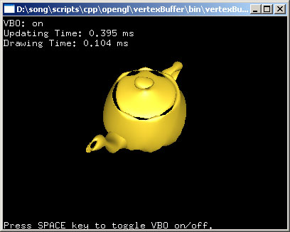
This demo application makes a VBO wobbling in and out along normals. It maps a VBO and updates its vertices every frame with the pointer to the mapped buffer. You can compare the performace with a traditional vertex array implementation.

It uses 2 vertex buffers; one for both vertex coords and normals, and the other stores index array only.

Download the source and binary: vbo.zip, vboSimple.zip.

vboSimple is a very simple example to draw a cube using VBO and Vertex Array. You can easily see what is common and what is different between VBO and VA.

I also include a makefile (Makefile.linux) for linux system in src folder, so you can build an executable on your linux box, for example:

This unofficial AutoCAD history site is a service to fellow users and trivia aficionados.

This site includes detailed command and system variables that have changed with each release and even some screen shots of old release material.

Regards,
Shaan Hurley
shaan.hurley@autodesk.com

AutoCAD DWG Version History by Release for the past 20+ years
The first six bytes of a DWG file identify its version. In a DXF file, the AutoCAD version number is specified in the header section. The DXF system variable is $ACADVER.

AutoCAD 2008 can read DWG files back from AutoCAD version 2.0 released in 1984.

Shadow volumes are a technique used in 3D computer graphics to add shadows to a rendered scene. They were first proposed by Frank Crow in 1977^[1] as the geometry describing the 3D shape of the region occluded from a light source. A shadow volume divides the virtual world in two: areas that are in shadow and areas that are not.

The stencil buffer implementation of shadow volumes is generally considered among the most practical general purpose real-time shadowing techniques utilizing the capabilities of modern 3D graphics hardware. It has been popularized by the computer game Doom 3, and a particular variation of the technique used in this game has become known as Carmack's Reverse (see depth fail below).

This technique as well as shadow mapping has become popular real-time shadowing techniques. The main advantage of shadow volumes is that they are accurate to the pixel (though many implementations have a minor self-shadowing problem along the silhouette edge, see construction below), whereas the accuracy of a shadow map depends on the texture memory allotted to it as well as the angle at which the shadows are cast (at some angles, the accuracy of a shadow map unavoidably suffers). However, the shadow volume technique requires the creation of shadow geometry, which can be CPU intensive (depending on the implementation). The advantage of shadow mapping is that it is often faster, the reason for which is that shadow volume polygons are often very large in terms of screen space and require a lot of fill time (especially for convex objects), whereas shadow maps do not have this limitation.

[edit] Construction

In order to construct a shadow volume, project a ray from the light through each vertex in the shadow casting object to some point (generally at infinity). These projections will together form a volume; any point inside that volume is in shadow, everything outside is lit by the light.

For a polygonal model, the volume is usually formed by classifying each face in the model as either facing toward the light source or facing away from the light source. The set of all edges that connect a toward-face to an away-face form the silhouette with respect to the light source. The edges forming the silhouette are extruded away from the light to construct the faces of the shadow volume. This volume must extend over the range of the entire visible scene; often the dimensions of the shadow volume are extended to infinity to accomplish this (see optimization below.) To form a closed volume, the front and back end of this extrusion must be covered. These coverings are called "caps". Depending on the method used for the shadow volume, the front end may be covered by the object itself, and the rear end may sometimes be omitted (see depth pass below).

There is also a problem with the shadow where the faces along the silhouette edge are relatively shallow. In this case, the shadow an object casts on itself will be sharp, revealing its polygonal facets, whereas the usual lighting model will have a gradual change in the lighting along the facet. This leaves a rough shadow artifact near the silhouette edge which is difficult to correct. Increasing the polygonal density will minimize the problem, but not eliminate it. If the front of the shadow volume is capped, the entire shadow volume may be offset slightly away from the light to remove any shadow self-intersections within the offset distance of the silhouette edge (this solution is more commonly used in shadow mapping).

The basic steps for forming a shadow volume are:

1. Find all silhouette edges (edges which separate front-facing faces from back-facing faces)
2. Extend all silhouette edges in the direction away from the light-source
3. Add a front-cap and/or back-cap to each surface to form a closed volume (may not be necessary, depending on the implementation used)

[edit] Stencil buffer implementations

After Crow, Tim Heidmann showed in 1991 how to use the stencil buffer to render shadows with shadow volumes quickly enough for use in real time applications. There are three common variations to this technique, depth pass, depth fail, and exclusive-or, but all of them use the same process:

1. Render the scene as if it were completely in shadow.
2. For each light source:
   1. Using the depth information from that scene, construct a mask in the stencil buffer that has holes only where the visible surface is not in shadow.
   2. Render the scene again as if it were completely lit, using the stencil buffer to mask the shadowed areas. Use additive blending to add this render to the scene.

The difference between these three methods occurs in the generation of the mask in the second step. Some involve two passes, and some only one; some require less precision in the stencil buffer. (These algorithms function well in both OpenGL and Direct3D.)

Shadow volumes tend to cover large portions of the visible scene, and as a result consume valuable rasterization time (fill time) on 3D graphics hardware. This problem is compounded by the complexity of the shadow casting objects, as each object can cast its own shadow volume of any potential size onscreen. See optimization below for a discussion of techniques used to combat the fill time problem.

[edit] Depth pass

Heidmann proposed that if the front surfaces and back surfaces of the shadows were rendered in separate passes, the number of front faces and back faces in front of an object can be counted using the stencil buffer. If an object's surface is in shadow, there will be more front facing shadow surfaces between it and the eye than back facing shadow surfaces. If their numbers are equal, however, the surface of the object is not in shadow. The generation of the stencil mask works as follows:

1. Disable writes to the depth and colour buffers.
2. Use back-face culling.
3. Set the stencil operation to increment on depth pass (only count shadows in front of the object).
4. Render the shadow volumes (because of culling, only their front faces are rendered).
5. Use front-face culling.
6. Set the stencil operation to decrement on depth pass.
7. Render the shadow volumes (only their back faces are rendered).

After this is accomplished, all lit surfaces will correspond to a 0 in the stencil buffer, where the numbers of front and back surfaces of all shadow volumes between the eye and that surface are equal.

This approach has problems when the eye itself is inside a shadow volume (for example, when the light source moves behind an object). From this point of view, the eye sees the back face of this shadow volume before anything else, and this adds a −1 bias to the entire stencil buffer, effectively inverting the shadows. This can be remedied by adding a "cap" surface to the front of the shadow volume facing the eye, such as at the front clipping plane. There is another situation where the eye may be in the shadow of a volume cast by an object behind the camera, which also has to be capped somehow to prevent a similar problem. In most common implementations, because properly capping for depth-pass can be difficult to accomplish, the depth-fail method (see below) may be licensed for these special situations. Alternatively one can give the stencil buffer a +1 bias for every shadow volume the camera is inside, though doing the detection can be slow.

There is another potential problem if the stencil buffer does not have enough bits to accommodate the number of shadows visible between the eye and the object surface, because it uses saturation arithmetic. (If they used arithmetic overflow instead, the problem would be insignificant.)

Depth pass testing is also known as z-pass testing, as the depth buffer is often referred to as the z-buffer.

[edit] Depth fail

Around 2000, several people discovered that Heidmann's method can be made to work for all camera positions by reversing the depth. Instead of counting the shadow surfaces in front of the object's surface, the surfaces behind it can be counted just as easily, with the same end result. This solves the problem of the eye being in shadow, since shadow volumes between the eye and the object are not counted, but introduces the condition that the rear end of the shadow volume must be capped, or shadows will end up missing where the volume points backward to infinity.

1. Disable writes to the depth and colour buffers.
2. Use front-face culling.
3. Set the stencil operation to increment on depth fail (only count shadows behind the object).
4. Render the shadow volumes.
5. Use back-face culling.
6. Set the stencil operation to decrement on depth fail.
7. Render the shadow volumes.

The depth fail method has the same considerations regarding the stencil buffer's precision as the depth pass method. Also, similar to depth pass, it is sometimes referred to as the z-fail method.

William Bilodeau and Michael Songy discovered this technique in October 1998, and presented the technique at Creativity, a Creative Labs developer's conference, in 1999[1]. Sim Dietrich presented this technique at a Creative Labs developer's forum in 1999 [2]. A few months later, William Bilodeau and Michael Songy filed a US patent application for the technique the same year, US patent 6384822, entitled "Method for rendering shadows using a shadow volume and a stencil buffer" issued in 2002. John Carmack of id Software independently discovered the algorithm in 2000 during the development of Doom 3 [3]. Since he advertised the technique to the larger public, it is often known as Carmack's Reverse.

Bilodeau and Songy assigned their patent ownership rights to Creative Labs. Creative Labs, in turn, granted id Software a license to use the invention free of charge in exchange for future support of EAX technology. [4]

[edit] Exclusive-Or

Either of the above types may be approximated with an Exclusive-Or variation, which does not deal properly with intersecting shadow volumes, but saves one rendering pass (if not fill time), and only requires a 1-bit stencil buffer. The following steps are for the depth pass version:

1. Disable writes to the depth and colour buffers.
2. Set the stencil operation to XOR on depth pass (flip on any shadow surface).
3. Render the shadow volumes.

[edit] Optimization

• One method of speeding up the shadow volume geometry calculations is to utilize existing parts of the rendering pipeline to do some of the calculation. For instance, by using homogeneous coordinates, the w-coordinate may be set to zero to extend a point to infinity. This should be accompanied by a viewing frustum that has a far clipping plane that extends to infinity in order to accommodate those points, accomplished by using a specialized projection matrix. This technique reduces the accuracy of the depth buffer slightly, but the difference is usually negligible. Please see SIGGRAPH 2002 paper Practical and Robust Stenciled Shadow Volumes for Hardware-Accelerated Rendering, C. Everitt and M. Kilgard, for a detailed implementation.

• Rasterization time of the shadow volumes can be reduced by using an in-hardware scissor test to limit the shadows to a specific onscreen rectangle.

• NVIDIA has implemented a hardware capability called the depth bounds test that is designed to remove parts of shadow volumes that do not affect the visible scene. (This has been available since the GeForce FX 5900 model.) A discussion of this capability and its use with shadow volumes was presented at the Game Developers Conference in 2005. [5]

• Since the depth-fail method only offers an advantage over depth-pass in the special case where the eye is within a shadow volume, it is preferable to check for this case, and use depth-pass wherever possible. This avoids both the unnecessary back-capping (and the associated rasterization) for cases where depth-fail is unnecessary, as well as the problem of appropriately front-capping for special cases of depth-pass.

[edit] See also

• Silhouette edge
• Shadow mapping, an alternative shadowing algorithm
• Stencil buffer
• Depth buffer
• List of software patents

[edit] External links

• The Theory of Stencil Shadow Volumes
• The Mechanics of Robust Stencil Shadows
• An Introduction to Stencil Shadow Volumes
• Shadow Mapping and Shadow Volumes
• Stenciled Shadow Volumes in OpenGL
• Volume shadow tutorial
• Fast shadow volumes at NVIDIA
• Robust shadow volumes at NVIDIA
• Advanced Stencil Shadow and Penumbral Wedge Rendering

[edit] Regarding depth-fail patents

• "Creative Pressures id Software With Patents". Slashdot (July 28, 2004). Retrieved on 2006-05-16.
• "Creative patents Carmack's reverse". The Tech Report (July 29, 2004). Retrieved on 2006-05-16.
• "Creative gives background to Doom III shadow story". The Inquirer (July 29, 2004). Retrieved on 2006-05-16.

[edit] References

In computer graphics, a silhouette edge on a 3D body projected onto a 2D plane (display plane) is the collection of points whose outwards surface normal is perpendicular to the view vector. Due to discontinities in the surface normal, a silhouette edge is also an edge which separates a front facing face from a back facing face. Without loss of generality, this edge is usually chosen to be the closest one on a face, so that in parallel view this edge corresponds to the same one in a perspective view. Hence, if there is an edge between a front facing face and a side facing face, and another edge between a side facing face and back facing face, the closer one is chosen. The easy example is looking at a cube in the direction where the face normal is colinear with the view vector.

The first type of silhouette edge is sometimes troublesome to handle because it does not necessarily correspond to a physical edge in the CAD model. The reason that this can be an issue is that a programmer might corrupt the original model by introducing the new silhouette edge into the problem. Also, given that the edge strongly depends upon the orientation of the model and view vector, this can introduce numerical instablities into the algorithm (such as when a trick like dilution of precision is considered).

[edit] Computation

To determine the silhouette edge of an object, we first have to know the plane equation of all faces. Then, by examining the sign of the point-plane distance from the light-source to each face

Using this result, we can determine if the face is front- or back facing.

The silhouette edge(s) consist of all edges separating a front facing face from a back facing face.

A convenient and practical implementation of front/back facing detection is to use the unit normal of the plane (which is commonly precomputed for lighting effects anyhow), then simply applying the dot product of the light position to the plane's unit normal:

Note: The homogeneous coordinates, w and d, are not always needed for this computation.

This is also the technique used in the 2002 SIGGRAPH paper, "Practical and Robust Stenciled Shadow Volumes for Hardware-Accelerated Rendering"

[edit] External links

• http://wheger.tripod.com/vhl/vhl.htm

http://ati.amd.com/products/RadeonX1950/reviews.html

Scott Wasson, The Tech Report:
“I'd most likely pick the Radeon X1950 Pro for use in my own system. Nvidia's iffy texture filtering becomes really bothersome in games like Oblivion and Guild Wars, and since the X1950 Pro only pulls about 15W more under load than the 7900 GS, why not grab it instead? Also, we've been down this road half a dozen times in the past month, but it bears repeating that the Radeon X1000 series has some feature advantages that translate into better image quality than what Nvidia's G71 can offer, including smarter, more flexible antialiasing and angle-independent anisotropic filtering.”

Kurtis Kronk, Tech Lounge:
“Worth noting is that ATI still has the advantage of HDR+AA rendering over NVIDIA's current cards which don't support this. They also have WHQL certified drivers for Vista, with the X1950 Pro capable of providing a 'premium' level experience. NVIDIA does not. The Vista drivers aren't all that important to me at the moment, but it does bode well for ATI's driver team. Some people criticize ATI's driver team (particularly for the sluggish Catalyst Control Center), but I personally like that they have a driver release schedule and stick to it.”

Brandon Bell, FiringSquad:
““Connectivity options on ATI’s Radeon X1950 Pro are quite robust, particularly for a mainstream card at the $200 price point. Not only do you get two dual-link DVI connectors, ATI’s X1950 Pro also includes VIVO (video-in/video-out) support. Even NVIDIA’s $400 GeForce 7900 GTX doesn’t support VIVO.”

“With the Radeon X1950 Pro, ATI has essentially taken the basic ingredients found in the base Radeon X1900 GT, namely its 36 pixel shader/8 vertex shader architecture and spiced the package up a little further with faster memory speeds, a better cooler that runs very quiet, and for dual-GPU enthusiasts, integrated CrossFire support.”

Jason Cross, ExtremeTech:
“Today, ATI makes available a new midrange graphics card based on a new graphics chip dubbed R570. The Radeon X1950 Pro, targeted at a $199 retail price, is meant to offer better price/performance than anything else in its class, naturally. That's good news for budget-minded gamers, but the really exciting part is this: The Radeon X1950 Pro is the first GPU from ATI to incorporate a whole new CrossFire solution, with no more master cards, no more awkward external connectors, and an eye toward future scalability.”

“As a single card, the X1950 Pro is a real winner. It's a single slot card with plenty of DX9 shading power and performance, easily besting the GeForce 7900 GS in practically all our benchmarks—typically by 15% to 25%. If you're only interested in buying a single $200 graphics card, the X1950 Pro is the way to go. Note also, that it will support the GPU-accelerated Folding@Home project.”

Ryan Shrout, PC Perspective:
“If there is one place where ATI's CrossFire has had the advantage over NVIDIA's SLI multi-GPU technology, it is in platform support.  CrossFire will run on any of the CrossFire-ready ATI chipsets for AMD or Intel platforms, as well as the Intel 975X chipset (and recently the P965 chipset).”

“The Radeon X1950 Pro was definitely the best performing card for under $200; the majority our gaming tests showed that the X1950 Pro had the power to out perform the only a few months old NVIDIA 7900 GS card, even in the overclocked card we had from XFX.  In the pair of games where the X1950 Pro didn't win out right, the NVIDIA and ATI GPUs were neck and neck in performance at both 1600x1200 and 1920x1200.”

Brent Justice, HardOCP:
“ATI has come with a flurry of punches lately trying to take back the “video card crown” at very affordable price points. They started by introducing the Radeon X1950 XTX (the fastest single-GPU video card you can get) at only $450 MSRP. With today’s announcement ATI is poised to take the $199 pricing segment as well. The Radeon X1950 Pro performs exceptionally well for the price; it competes easily with NVIDIA’s GeForce 7900 GS providing a better experience in most games.”

Tarinder Sandhu, Hexus:
“The release of X1950 Pro changes the playing field in the crucial £125-£150 sector. It's priced at X1900 GT levels but augments the already decent specification with 'proper' CrossFire, HDCP support*, a quieter cooler, and, ultimately, better performance derived from greater memory bandwidth. If you liked the X1900 GT, the X1950 Pro offers more in every department for the same financial outlay, so what's already good is now better.”

Derek Wilson, AnandTech:
“There haven't been any changes to the way CrossFire works from an internal technical standpoint, but a handful of changes have totally revolutionized the way end users see CrossFire.”

“The bridge solution is much easier to work with than the external dongle, and while the 2 bridge solution is a little more cumbersome than a single bridge as with SLI, we can't argue with ATI's bridge distribution method or the fact that a 2 channel over the top connection offers greater flexibility in a more than 2 card multi-GPU solution. We also like the fact that ATI is distributing only flexible bridges as opposed to the more common PCB style bridges we often see on SLI systems.”

Brian Wallace, Legit Reviews:
“It's been a long hard road for CrossFire but ATI has finally released a GPU solution designed from the ground up to be used in Multi-GPU solutions and it shows. The X1950 Pro is a terrific introduction of what's to come from the red team in the near future. It's very encouraging to see such a polished product being launched because CrossFire is now one big step closer to SLI.”

“ATI delivers a well polished product, and most importantly, a great CrossFire experience to the mainstream market. With lower power usage, low heat output, and virtually no noise the X1950 Pro is the card many have been longing for.”

Bounding volume

From Wikipedia, the free encyclopedia

  (Redirected from K-DOP)

Jump to: navigation, search

A bounding box for a three dimensional model

For building code compliance, see Bounding.

In computer graphics and computational geometry, a bounding volume for a set of objects is a closed volume that completely contains the union of the objects in the set. Bounding volumes are used to improve the efficiency of geometrical operations by using simple volumes to contain more complex objects. Normally, simpler volumes have simpler ways to test for overlap.

A bounding volume for a set of objects is also a bounding volume for the single object consisting of their union, and the other way around. Therefore it is possible to confine the description to the case of a single object, which is assumed to be non-empty and bounded (finite).

Contents [hide] 1 Uses of bounding volumes 2 Common types of bounding volume 3 Basic intersection checks 4 See also 5 External links

[edit] Uses of bounding volumes

Bounding volumes are most often used to accelerate certain kinds of tests.

In ray tracing, bounding volumes are used in ray-intersection tests, and in many rendering algorithms, they are used for viewing frustum tests. If the ray or viewing frustum does not intersect the bounding volume, it cannot intersect the object contained in the volume. These intersection tests produce a list of objects that must be displayed. Here, displayed means rendered or rasterized.

In collision detection, when two bounding volumes do not intersect, then the contained objects cannot collide, either.

Testing against a bounding volume is typically much faster than testing against the object itself, because of the bounding volume's simpler geometry. This is because an 'object' is typically composed of polygons or data structures that are reduced to polygonal approximations. In either case, it is computationally wasteful to test each polygon against the view volume if the object is not visible. (Onscreen objects must be 'clipped' to the screen, regardless of whether their surfaces are actually visible.)

To obtain bounding volumes of complex objects, a common way is to break the objects/scene down using a scene graph or more specifically bounding volume hierarchies like e.g. OBB trees. The basic idea behind this is to organize a scene in a tree-like structure where the root comprises the whole scene and each leaf contains a smaller subpart.

[edit] Common types of bounding volume

The choice of the type of bounding volume for a given application is determined by a variety of factors: the computational cost of computing a bounding volume for an object, the cost of updating it in applications in which the objects can move or change shape or size, the cost of determining intersections, and the desired precision of the intesection test. It is common to use several types in conjunction, such as a cheap one for a quick but rough test in conjunction with a more precise but also more expensive type.

The types treated here all give convex bounding volumes. If the object being bounded is known to be convex, this is not a restriction. If non-convex bounding volumes are required, an approach is to represent them as a union of a number of convex bounding volumes. Unfortunately, intersection tests become quickly more expensive as the bounding boxes become more sophisticated.

A bounding sphere is a sphere containing the object. In 2-D graphics, this is a circle. Bounding spheres are represented by centre and radius. They are very quick to test for collision with each other: two spheres intersect when the distance between their centres does not exceed the sum of their radii. This makes bounding spheres appropriate for objects that can move in any number of dimensions.

A bounding ellipsoid is an ellipsoid containing the object. Ellipsoids usually provide tighter fitting than a sphere. Intersections with ellipsoids are done by scaling the other object along the principal axes of the ellipsoid by an amount equal to the multiplicative inverse of the radii of the ellipsoid, thus reducing the problem to intersecting the scaled object with a unit sphere. Care should be taken to avoid problems if the applied scaling introduces skew. Skew can make the usage of ellipsoids impractical in certain cases, for example collision between two arbitrary ellipsoids.

A bounding cylinder is a cylinder containing the object. In most applications the axis of the cylinder is aligned with the vertical direction of the scene. Cylinders are appropriate for 3-D objects that can only rotate about a vertical axis but not about other axes, and are otherwise constrained to move by translation only. Two vertical-axis-aligned cylinders intersect when, simultaneously, their projections on the vertical axis intersect – which are two line segments – as well their projections on the horizontal plane – two circular disks. Both are easy to test. In video games, bounding cylinders are often used as bounding volumes for people standing upright.

A bounding capsule is a swept sphere (i.e. the volume that a sphere takes as it moves along a straight line segment) containing the object. Capsules can be represented by the radius of the swept sphere and the segment that the sphere is swept across). It has traits similar to a cylinder, but is easier to use, because the intersection test is simpler. A capsule and another object intersect if the distance between the capsule's defining segment and some feature of the other object is smaller than the capsule's radius. For example, two capsules intersect if the distance between the capsules' segments is smaller than the sum of their radii. This holds for arbitrarily rotated capsules, which is why they're more appealing than cylinders in practice.

A bounding box is a cuboid, or in 2-D a rectangle, containing the object. In dynamical simulation, bounding boxes are preferred to other shapes of bounding volume such as bounding spheres or cylinders for objects that are roughly cuboid in shape when the intersection test needs to be fairly accurate. The benefit is obvious, for example, for objects that rest upon other, such as a car resting on the ground: a bounding sphere would show the car as possibly intersecting with the ground, which then would need to be rejected by a more expensive test of the actual model of the car; a bounding box immediately shows the car as not intersecting with the ground, saving the more expensive test.

In many applications the bounding box is aligned with the axes of the co-ordinate system, and it is then known as an axis-aligned bounding box (AABB). To distinguish the general case from an AABB, an arbitrary bounding box is sometimes called an oriented bounding box (OBB). AABBs are much simpler to test for intersection than OBBs, but have the disadvantage that when the model is rotated they cannot be simply rotated with it, but need to be recomputed.

A minimum bounding rectangle or MBR – the least AABB in 2-D – is frequently used in the description of geographic (or "geospatial") data items, serving as a simplified proxy for a dataset's spatial extent (see geospatial metadata) for the purpose of data search (including spatial queries as applicable) and display. It is also a basic component of the R-tree method of spatial indexing.

A discrete oriented polytope (DOP) generalizes the AABB. A DOP is a convex polytope containing the object (in 2-D a polygon; in 3-D a polyhedron), constructed by taking a number of suitably oriented planes at infinity and moving them until they collide with the object. The DOP is then the convex polytope resulting from intersection of the half-spaces bounded by the planes. Popular choices for constructing DOPs in 3-D graphics include the axis-aligned bounding box, made from 6 axis-aligned planes, and the beveled bounding box, made from 10 (if beveled only on vertical edges, say) 18 (if beveled on all edges), or 26 planes (if beveled on all edges and corners). A DOP constructed from k planes is called a k-DOP; the actual number of faces can be less than k, since some can become degenerate, shrunk to an edge or a vertex.

A convex hull is the smallest convex volume containing the object. If the object is the union of a finite set of points, its convex hull is a polytope, and in fact the smallest possible containing polytope.

[edit] Basic intersection checks

For some types of bounding volume (OBB and convex polyhedra), an effective check is that of the separating axis theorem. The idea here is that, if there exists an axis by which the objects do not overlap, then the objects do not intersect. Usually the axes checked are those of the basic axes for the volumes (the unit axes in the case of an AABB, or the 3 base axes from each OBB in the case of OBBs). Often, this is followed by also checking the cross-products of the previous axes (one axis from each object).

In the case of an AABB, this tests becomes a simple set of overlap tests in terms of the unit axes. For an AABB defined by M,N against one defined by O,P they do not intersect if (M_x>P_x) or (O_x>N_x) or (M_y>P_y) or (O_y>N_y) or (M_z>P_z) or (O_z>N_z).

An AABB can also be projected along an axis, for example, if it has edges of length L and is centered at C, and is being projected along the axis N:
, and or , and where m and n are the minimum and maximum extents.

An OBB is similar in this respect, but is slightly more complicated. For an OBB with L and C as above, and with I, J, and K as the OBB's base axes, then:

For the ranges m,n and o,p it can be said that they do not intersect if m>p or o>n. Thus, by projecting the ranges of 2 OBBs along the I, J, and K axes of each OBB, and checking for non-intersection, it is possible to detect non-intersection. By additionally checking along the cross products of these axes (I₀×I₁, I₀×J₁, ...) one can be more certain that intersection is impossible.

This concept of determining non-intersection via use of axis projection also extends to convex polyhedra, however with the normals of each polyhedral face being used instead of the base axes, and with the extents being based on the minimum and maximum dot products of each vertex against the axes. Note that this description assumes the checks are being done in world space.

[edit] See also

• Minimum bounding rectangle
• Spatial index
• Minimum bounding box

[edit] External links

• Illustration of several DOPs for the same model, from epicgames.com

Retrieved from "http://en.wikipedia.org/wiki/Bounding_volume"

Collision detection

From Wikipedia, the free encyclopedia

Jump to: navigation, search

For collision detection on networks see CSMA/CD

In physical simulations, video games and computational geometry, collision detection involves algorithms for checking for collision, i.e. intersection, of two given solids. Simulating what happens once a collision is detected is sometimes referred to as "collision response", for which see physics engine and ragdoll physics. Collision detection algorithms are a basic component of 3D video games. Without them, characters could go through walls and other obstacles.

Contents [hide] 1 Overview 2 Collision detection in physical simulation 2.1 A posteriori versus a priori 3 Optimization 3.1 Exploiting temporal coherence 3.2 Pairwise pruning 3.3 Exact pairwise collision detection 3.4 A priori pruning 3.5 Spatial partitioning 4 Video games 5 Open Source Collision Detection 6 References 7 See also 8 External links

[edit] Overview

Billiards balls hitting each other are a classic example applicable within the science of collision detection.

In physical simulation, we wish to conduct experiments, such as playing billiards. The physics of bouncing billiard balls are well understood, under the umbrella of rigid body motion and elastic collisions. An initial description of the situation would be given, with a very precise physical description of the billiard table and balls, as well as initial positions of all the balls. Given a certain impulsion on the cue ball (probably resulting from a player hitting the ball with his cue stick), we want to calculate the trajectories, precise motion, and eventual resting places of all the balls with a computer program. A program to simulate this game would consist of several portions, one of which would be responsible for calculating the precise impacts between the billiard balls. This particular example also turns out to be numerically unstable: a small error in any calculation will cause drastic changes in the final position of the billiard balls.

Video games have similar requirements, with some crucial differences. While physical simulation needs to simulate real-world physics as precisely as possible, video games need to simulate real-world physics in an acceptable way, in real time and robustly. Compromises are allowed, so long as the resulting simulation is satisfying to the game player.

[edit] Collision detection in physical simulation

Physical simulators differ in the way they react on a collision. Some use the softness of the material to calculate a force, which will resolve the collision in the following time steps like it is in reality. Due to the low softness of some materials this is very CPU intensive. Some simulators estimate the time of collision by linear interpolation, roll back the simulation, and calculate the collision by the more abstract methods of conservation laws.

Some iterate the linear interpolation (Newton's method) to calculate the time of collision with a much higher precision than the rest of the simulation. Collision detection utilizes time coherence to allow ever finer time steps without much increasing CPU demand, such as in air traffic control.

After an inelastic collision, special states of sliding and resting can occur and, for example, the Open Dynamics Engine uses constrains to simulate them. Constrains avoid inertia and thus instability. Implementation of rest by means of a scene graph avoids drift.

In other words, physical simulators usually function one of two ways, where the collision is detected a posteriori (after the collision occurs) or a priori (before the collision occurs). In addition to the a posteriori and a priori distinction, almost all modern collision detection algorithms are broken into a hierarchy of algorithms.

[edit] A posteriori versus a priori

In the a posteriori case, we advance the physical simulation by a small time step, then check if any objects are intersecting, or are somehow so close to each other that we deem them to be intersecting. At each simulation step, a list of all intersecting bodies is created, and the positions and trajectories of these objects are somehow "fixed" to account for the collision. We say that this method is a posteriori because we typically miss the actual instant of collision, and only catch the collision after it has actually happened.

In the a priori methods, we write a collision detection algorithm which will be able to predict very precisely the trajectories of the physical bodies. The instants of collision are calculated with high precision, and the physical bodies never actually interpenetrate. We call this a priori because we calculate the instants of collision before we update the configuration of the physical bodies.

The main benefits of the a posteriori methods are as follows. In this case, the collision detection algorithm need not be aware of the myriad physical variables; a simple list of physical bodies is fed to the algorithm, and the program returns a list of intersecting bodies. The collision detection algorithm doesn't need to understand friction, elastic collisions, or worse, nonelastic collisions and deformable bodies. In addition, the a posteriori algorithms are in effect one dimension simpler than the a priori algorithms. Indeed, an a priori algorithm must deal with the time variable, which is absent from the a posteriori problem.

On the other hand, a posteriori algorithms cause problems in the "fixing" step, where intersections (which aren't physically correct) need to be corrected. In fact, there are some^[who?] who believe that such an algorithm is inherently flawed and unstable^{[citation needed]}.

The benefits of the a priori algorithms are increased fidelity and stability. It is difficult (but not completely impossible) to separate the physical simulation from the collision detection algorithm. However, in all but the simplest cases, the problem of determining ahead of time when two bodies will collide (given some initial data) has no closed form solution -- a numerical root finder is usually involved.

Some objects are in resting contact, that is, in collision, but neither bouncing off, nor interpenetrating, such as a vase resting on a table. In all cases, resting contact requires special treatment: If two objects collide (a posteriori) or slide (a priori) and their relative motion is below a threshold, friction becomes stiction and both objects are arranged in the same branch of the scene graph; however, some believe that it poses special problems in a posteriori algorithm^{[citation needed]}.

[edit] Optimization

The obvious approaches to collision detection for multiple objects are very slow. Checking every object against every other object will, of course, work, but is too inefficient to be used when the number of objects is at all large. Checking objects with complex geometry against each other in the obvious way, by checking each face against each other face, is itself quite slow. Thus, considerable research has been applied to speeding up the problem.

[edit] Exploiting temporal coherence

In many applications, the configuration of physical bodies from one time step to the next changes very little. Many of the objects may not move at all. Algorithms have been designed so that the calculations done in a preceding time step can be reused in the current time step, resulting in faster algorithms.

At the coarse level of collision detection, the objective is to find pairs of objects which might potentially intersect. Those pairs will require further analysis. An early high performance algorithm for this was developed by M. C. Lin at U.C. Berkley [1], who suggested using axis-aligned bounding boxes for all n bodies in the scene.

Each box is represented by the product of three intervals (i.e., a box would be .) A common algorithm for collision detection of bounding boxes is sweep and prune. We observe that two such boxes, and intersect if, and only if, I₁ intersects J₁, I₂ intersects J₂ and I₃ intersects J₃. We suppose that, from one time step to the next, I_k and J_k intersect, then it is very likely that at the next time step, they will still intersect. Likewise, if they did not intersect in the previous time step, then they are very likely to continue not to.

So we reduce the problem to that of tracking, from frame to frame, which intervals do intersect. We have three lists of intervals (one for each axis) and all lists are the same length (since each list has length n, the number of bounding boxes.) In each list, each interval is allowed to intersect all other intervals in the list. So for each list, we will have an matrix M = (m_ij) of zeroes and ones: m_ij is 1 if intervals i and j intersect, and 0 if they do not intersect.

By our assumption, the matrix M associated to a list of intervals will remain essentially unchanged from one time step to the next. To exploit this, the list of intervals is actually maintained as a list of labeled endpoints. Each element of the list has the coordinate of an endpoint of an interval, as well as a unique integer identifying that interval. Then, we sort the list by coordinates, and update the matrix M as we go. It's not so hard to believe that this algorithm will work relatively quickly if indeed the configuration of bounding boxes does not change significantly from one time step to the next.

In the case of deformable bodies such as cloth simulation, it may not be possible to use a more specific pairwise pruning algorithm as discussed below, and an n-body pruning algorithm is the best that can be done.

If an upper bound can be placed on the velocity of the physical bodies in a scene, then pairs of objects can be pruned based on their initial distance and the size of the time step.

[edit] Pairwise pruning

Once we've selected a pair of physical bodies for further investigation, we need to check for collisions more carefully. However, in many applications, individual objects (if they are not too deformable) are described by a set of smaller primitives, mainly triangles. So now, we have two sets of triangles, and (for simplicity, we will assume that each set has the same number of triangles.)

The obvious thing to do is to check all triangles S_j against all triangles T_k for collisions, but this involves n² comparisons, which is highly inefficient. If possible, it is desirable to use a pruning algorithm to reduce the number of pairs of triangles we need to check.

The most widely used family of algorithms is known as the hierarchical bounding volumes method. As a preprocessing step, for each object (in our example, S and T) we will calculate a hierarchy of bounding volumes. Then, at each time step, when we need to check for collisions between S and T, the hierarchical bounding volumes are used to reduce the number of pairs of triangles under consideration. For the sake of simplicity, we will give an example using bounding spheres, although it has been noted that spheres are undesirable in many cases.^{[citation needed]}

If E is a set of triangles, we can precalculate a bounding sphere B(E). There are many ways of choosing B(E), we only assume that B(E) is a sphere that completely contains E and is as small as possible.

Ahead of time, we can compute B(S) and B(T). Clearly, if these two spheres do not intersect (and that is very easy to test,) then neither do S and T. This is not much better than an n-body pruning algorithm, however.

If is a set of triangles, then we can split it into two halves and . We can do this to S and T, and we can calculate (ahead of time) the bounding spheres B(L(S)),B(R(S)) and B(L(T)),B(R(T)). The hope here is that these bounding spheres are much smaller than B(S) and B(T). And, if, for instance, B(S) and B(L(T)) do not intersect, then there is no sense in checking any triangle in S against any triangle in L(T).

As a precomputation, we can take each physical body (represented by a set of triangles) and recursively decompose it into a binary tree, where each node N represents a set of triangles, and its two children represent L(N) and R(N). At each node in the tree, as a we can precompute the bounding sphere B(N).

When the time comes for testing a pair of objects for collision, their bounding sphere tree can be used to eliminate many pairs of triangles.

Many variants of the algorithms are obtained by choosing something other than a sphere for B(T). If one chooses axis-aligned bounding boxes, one gets AABBTrees. Oriented bounding box trees are called OBBTrees. Some trees are easier to update if the underlying object changes. Some trees can accommodate higher order primitives such as splines instead of simple triangles.

[edit] Exact pairwise collision detection

Once we're done pruning, we are left with a number of candidate pairs to check for exact collision detection.

A basic observation is that for any two convex objects which are disjoint, one can find a plane in space so that one object lies completely on one side of that plane, and the other object lies on the opposite side of that plane. This allows the development of very fast collision detection algorithms for convex objects.

Early work in this area involved "separating plane" methods. Two triangles collide essentially only when they can not be separated by a plane going through three vertices. That is, if the triangles are v₁,v₂,v₃ and v₄,v₅,v₆ where each v_j is a vector in , then we can take three vertices, v_i,v_j,v_k, find a plane going through all three vertices, and check to see if this is a separating plane. If any such plane is a separating plane, then the triangles are deemed to be disjoint. On the other hand, if none of these planes are separating planes, then the triangles are deemed to intersect. There are twenty such planes.

If the triangles are coplanar, this test is not entirely successful. One can either add some extra planes, for instance, planes that are normal to triangle edges, to fix the problem entirely. In other cases, objects that meet at a flat face must necessarily also meet at an angle elsewhere, hence the overall collision detection will be able to find the collision.

Better methods have since been developed. Very fast algorithms are available for finding the closest points on the surface of two convex polyhedral objects. Early work by M. C. Lin ^[1] used a variation on the simplex algorithm from linear programming. The Gilbert-Johnson-Keerthi distance algorithm has superseded that approach. These algorithms approach constant time when applied repeatedly to pairs of stationary or slow-moving objects, when used with starting points from the previous collision check.

The end result of all this algorithmic work is that collision detection can be done efficiently for thousands of moving objects in real time on typical personal computers and game consoles.

[edit] A priori pruning

Where most of the objects involved are fixed, as is typical of video games, a priori methods using precomputation can be used to speed up execution.

Pruning is also desirable here, both n-body pruning and pairwise pruning, but the algorithms must take time and the types of motions used in the underlying physical system into consideration.

When it comes to the exact pairwise collision detection, this is highly trajectory dependent, and one almost has to use a numerical root-finding algorithm to compute the instant of impact.

As an example, consider two triangles moving in time v₁(t),v₂(t),v₃(t) and v₄(t),v₅(t),v₆(t). At any point in time, the two triangles can be checked for intersection using the twenty planes previously mentioned. However, we can do better, since these twenty planes can all be tracked in time. If P(u,v,w) is the plane going through points u,v,w in then there are twenty planes P(v_i(t),v_j(t),v_k(t)) to track. Each plane needs to be tracked against three vertices, this gives sixty values to track. Using a root finder on these sixty functions produces the exact collision times for the two given triangles and the two given trajectory. We note here that if the trajectories of the vertices are assumed to be linear polynomials in t then the final sixty functions are in fact cubic polynomials, and in this exceptional case, it is possible to locate the exact collision time using the formula for the roots of the cubic. Some numerical analysts suggest that using the formula for the roots of the cubic is not as numerically stable as using a root finder for polynomials.^{[citation needed]}

[edit] Spatial partitioning

Alternative algorithms are grouped under the spatial partitioning umbrella, which includes octrees, binary space partitioning (or BSP trees) and other, similar approaches. If one splits space into a number of simple cells, and if two objects can be shown not to be in the same cell, then they need not be checked for intersection. Since BSP trees can be precomputed, that approach is well suited to handling walls and fixed obstacles in games. These algorithms are generally older than the algorithms described above.

[edit] Video games

Video games have to split their very limited computing time between several tasks. Despite this resource limit, and the use of relatively primitive collision detection algorithms, programmers have been able to create believeable, if inexact, systems for use in games.

For a long time, video games had a very limited number of objects to treat, and so checking all pairs was not a problem. In two-dimensional games, in some cases, the hardware was able to efficiently detect and report overlapping pixels between sprites on the screen. In other cases, simply tiling the screen and binding each sprite into the tiles it overlaps provides sufficient pruning, and for pairwise checks, bounding rectangles or circles are used and deemed sufficiently accurate.

Three dimensional games have used spatial partitioning methods for n-body pruning, and for a long time used one or a few spheres per actual 3D object for pairwise checks. Exact checks are very rare, except in games attempting to simulate reality closely. Even then, exact checks are not necessarily used in all cases.

Because games use simplified physics, stability is not as much of an issue.^{[citation needed]} Almost all games use a posteriori collision detection, and collisions are often resolved using very simple rules. For instance, if a character becomes embedded in a wall, he might be simply moved back to his last known good location. Some games will calculate the distance the character can move before getting embedded into a wall, and only allow him to move that far.

A slightly more sophisticated and striking effect is ragdoll physics. If a video game character is disabled, instead of playing a preset animation, a simplified skeleton of the character is animated as if it were a rag doll. This rag doll falls limp, and might collide with itself and the environment, in which case it should behave appropriately.

In many cases for video games, approximating the characters by a point is sufficient for the purpose of collision detection with the environment. In this case, binary space partition trees provide a viable, efficient and simple algorithm for checking if a point is embedded in the scenery or not. Such a data structure can also be used to handle "resting position" situation gracefully when a character is running along the ground. Collisions between characters, and collisions with projectiles and hazards, are treated separately.

A robust simulator is one that will react to any input in a reasonable way. For instance, if we imagine a high speed racecar video game, from one simulation step to the next, it is conceivable that the cars would advance a substantial distance along the race track. If there is a shallow obstacle on the track (such as a brick wall), it is not entirely unlikely that the car will completely leap over it, and this is very undesirable. In other instances, the "fixing" that the a posteriori algorithms require isn't implemented correctly, and characters find themselves embedded in walls, or falling off into a deep black void. These are the hallmarks of a mediocre collision detection and physical simulation system.

[edit] Open Source Collision Detection

• GJKD A 2D implementation of the Gilbert-Johnson-Keerthi (GJK) algorithm, written in D.
• MPR2D A 2D implementation of the Minkowski Portal Refinement (MPR) Algorithm, written in D.

[edit] References

1. ^ Lin, Ming C. "Efficient Collision Detection for Animation and Robotics (thesis)". University of California, Berkeley.

[edit] See also

• Bounding volume
• Game physics
• Gilbert–Johnson–Keerthi distance algorithm
• Physics engine
• Ragdoll physics

[edit] External links

• University of California, Berkeley collision detection research web site
• Prof. Steven Cameron (Oxford University) web site on collision detection
• How to Avoid a Collision by George Beck, The Wolfram Demonstrations Project.
• Basic collision detection in OpenGL.

Retrieved from "http://en.wikipedia.org/wiki/Collision_detection"

http://gamasutra.com/features/20000807/kovach_01.htm
Inside Direct3D: Stencil Buffers

One aspect of advanced rendering we haven't discussed yet is stenciling, a technique that can be useful for developing commercial applications. If you want your 3D applications to stand apart from the crowd, you'd be wise to combine stenciling with the texturing techniques you learned about in earlier chapters. This chapter will detail how to use stenciling and show you the different types of effects you can generate with it.

Many 3D games and simulations on the market use cinema-quality special effects to add to their dramatic impact. You can use stencil buffers to create effects such as composites, decals, dissolves, fades, outlines, silhouettes, swipes, and shadows. Stencil buffers determine whether the pixels in an image are drawn. To perform this function, stencil buffers let you enable or disable drawing to the render-target surface on a pixel-by-pixel basis. This means your software can "mask" portions of the rendered image so that they aren't displayed.

When the stenciling feature is enabled, Microsoft Direct3D performs a stencil test for each pixel that it plans to write to the render-target surface. The stencil test uses a stencil reference value, a stencil mask, a comparison function, and a pixel value from the stencil buffer that corresponds to the current pixel in the target surface. Here are the specific steps used in this test:

1. Perform a bitwise AND operation of the stencil reference value with the stencil mask.
2. Perform a bitwise AND operation on the stencil-buffer value for the current pixel with the stencil mask.
3. Compare the results of Step 1 and Step 2 by using the comparison function.

By controlling the comparison function, the stencil mask, the stencil reference value, and the action taken when the stencil test passes or fails, you can control how the stencil buffer works. As long as the test succeeds, the current pixel will be written to the target. The default comparison behavior (the value that the D3DCMPFUNC enumerated type defines for D3DCMP_ALWAYS) is to write the pixel without considering the contents of the stencil buffer. You can change the comparison function to any function you want by setting the value of the D3DRENDERSTATE_STENCILFUNC render state and passing one of the members of the D3DCMPFUNC enumerated type.

Creating a Stencil Buffer

Before creating a stencil buffer, you need to determine what stenciling capabilities the target system supports. To do this, call the IDirect3DDevice7::GetCaps method. The dwStencilCaps flags specify the stencil-buffer operations that the device supports. The reported flags are valid for all three stencil-buffer operation render states: D3DRENDERSTATE_STENCILFAIL, D3DRENDERSTATE_STENCILPASS, and D3DRENDERSTATE_STENCILZFAIL. Direct3D defines the following flags for dwStencilCaps:

• D3DSTENCILCAPS_DECR Indicates that the D3DSTENCILOP_DECR operation is supported
  
  
• D3DSTENCILCAPS_DECRSAT Indicates that the D3DSTENCILOP_DECRSAT operation is supported
  
  
• D3DSTENCILCAPS_INCR Indicates that the
  D3DSTENCILOP_INCR operation is supported
  
  
• D3DSTENCILCAPS_INCRSAT Indicates that the D3DSTENCILOP_INCRSAT operation is supported
  
  
• D3DSTENCILCAPS_INVERT Indicates that the D3DSTENCILOP_INVERT operation is supported
  
  
• D3DSTENCILCAPS_KEEP Indicates that the D3DSTENCILOP_KEEP operation is supported
  
  
• D3DSTENCILCAPS_REPLACE Indicates that the D3DSTENCILOP_REPLACE operation is supported
  
  
• D3DSTENCILCAPS_ZERO Indicates that the D3DSTENCILOP_ZERO operation is supported
  

If the method succeeds, it returns the value D3D_OK. If it fails, the method returns one of these four values:

• DDERR_INVALIDOBJECT
  
  
• DDERR_INVALIDPARAMS
  
  
• DDER_NOZBUFFERHW
  
  
• DDERR_OUTOFMEMORY

The code in listing 1 determines what stencil buffer formats are available and what operations are supported and then creates a stencil buffer. As you can see, this code notes whether the stencil buffer supports more than 1-bit -- some stenciling techniques must be handled differently if only a 1-bit stencil buffer is available.

Clearing a Stencil Buffer

The IDirect3DDevice7 interface includes the Clear method, which you can use to simultaneously clear the render target's color buffer, depth buffer, and stencil buffer. Here's the declaration for the IDirect3DDevice7::Clear method:

    HRESULT IDirect3DDevice7::Clear(
       DWORD dwCount,
       LPD3DRECT lpRects,
       DWORD dwFlags,
       D3DVALUE dvZ,
       DWORD dwStencil
    );

The IDirect3DDevice7::Clear method still accepts the older D3DCLEAR_TARGET flag, which clears the render target using an RGBA color you provide in the dwColor parameter. This method also still accepts the D3DCLEAR_ZBUFFER flag, which clears the depth buffer to a depth you specify in dvZ (in which 0.0 is the closest distance and 1.0 is the farthest). DirectX 6 introduced the D3DCLEAR_STENCIL flag, which you can use to reset the stencil bits to the value you specify in the dwStencil parameter. This value can be an integer ranging from 0 to 2n-1, in which n is the bit depth of the stencil buffer.

________________________________________________________

Configuring the Stenciling State

Configuring the Stenciling State
You control the various settings for the stencil buffer using the IDirect3DDevice7::
SetRenderState method. Listing 2 shows the stencil-related members of the D3DRENDERSTATETYPE enumerated type.

      These are the definitions for the stencil-related render states:

• D3DRENDERSTATE_STENCILENABLE Use this member to enable or disable stenciling. To enable stenciling, use this member with TRUE; to disable stenciling, use it with FALSE. The default value is FALSE.
  
  
• D3DRENDERSTATE_STENCILFAIL Use this member to indicate the stencil operation to perform if the stencil test fails. The stencil operation can be one of the members of the D3DSTENCILOP enumerated type. The default value is D3DSTENCILOP_KEEP.
  
  
• D3DRENDERSTATE_STENCILZFAIL Use this member to indicate the stencil operation to perform if the stencil test passes and the depth test (z-test) fails. The operation can be one of the members of the D3DSTENCILOP enumerated type. The default value is D3DSTENCILOP_KEEP.
  
  
• D3DRENDERSTATE_STENCILPASS Use this member to indicate the stencil operation to perform if both the stencil test and the depth test (z-test) pass. The operation can be one of the members of the D3DSTENCILOP enumerated type. The default value is D3DSTENCILOP_KEEP.
  
  
• D3DRENDERSTATE_STENCILFUNC Use this member to indicate the comparison function for the stencil test. The comparison function can be one of the members of the D3DCMPFUNC enumerated type. The default value is D3DCMP_ALWAYS. This function compares the reference value to a stencil-buffer entry and applies only to the bits in the reference value and stencil-buffer entry that are set in the stencil mask. (The D3DRENDERSTATE_STENCILMASK render state sets the stencil mask.) If the comparison is true, the stencil test passes.
  
  
• D3DRENDERSTATE_STENCILREF Use this member to indicate the integer reference value for the stencil test. The default value is 0.
  
  
• D3DRENDERSTATE_STENCILMASK Use this member to specify the mask to apply to the reference value and each stencil-buffer entry to determine the significant bits for the stencil test. The default mask is 0xFFFFFFFF.
  
  
• D3DRENDERSTATE_STENCILWRITEMASK Use this member to specify the mask to apply to values written into the stencil buffer. The default mask is 0xFFFFFFFF.
  
  

The D3DSTENCILOP enumerated type describes the stencil operations for the D3DRENDERSTATE_STENCILFAIL, D3DRENDERSTATE_STENCILZFAIL, and D3DRENDERSTATE_STENCILPASS render states. Here's the definition of D3DSTENCILOP:

    //--------------------------------------------------
    // Name: RenderShadow
    // Desc:
    //------------------------------------------------
    HRESULT CMyD3DApplication::RenderShadow()
    {
        // Turn off depth buffer and turn on
           stencil buffer.
        m_pd3dDevice->SetRenderState(
                           D3DRENDERSTATE_ZWRITEENABLE,
                                     FALSE );
        m_pd3dDevice->SetRenderState(
                           D3DRENDERSTATE_STENCILENABLE,
                                     TRUE );

Next the code sets the comparison function that performs the stencil test by calling the IDirect3DDevice7::SetRenderState method and setting the first parameter to D3DRENDERSTATE_STENCILFUNC. The second parameter is set to a member of the D3DCMPFUNC enumerated type. In this code, we want to update the stencil buffer everywhere a primitive is rendered, so we use D3DCMP_ALWAYS:

     //
    // Set up stencil comparison function,
       reference value, and masks.
    // Stencil test passes if ((ref & mask)
       cmpfn (stencil & mask))
    // is true.
    //
    m_pd3dDevice->SetRenderState(
                           D3DRENDERSTATE_STENCILFUNC,
                                 D3DCMP_ALWAYS );

In this sample, we don't want the stencil buffer to change if either the stencil buffer test or the depth buffer test fails, so we set the appropriate states to D3DSTENCILOP_KEEP:

     m_pd3dDevice->SetRenderState(
                          D3DRENDERSTATE_STENCILZFAIL,
                                  D3DSTENCILOP_KEEP );
     m_pd3dDevice->SetRenderState(
                          D3DRENDERSTATE_STENCILFAIL,
                                  D3DSTENCILOP_KEEP );

The settings in listing 3 are different depending on whether a 1-bit or a multibit stencil buffer is present. If the stencil buffer has only 1 bit, the value 1 is stored in the stencil buffer whenever the stencil test passes. Otherwise, an increment operation (either D3DSTENCILOP_INCR or D3DSTENCILOP_INCRSAT) is applied if the stencil test passes. At this point, the stencil state is configured and the code is ready to render some primitives.

________________________________________________________

Creating Effects

Creating Effects
Now that you've seen how to create stencil buffers and configure how they work, let's look at some of the effects you can render with them. The following sections describe several ways Microsoft recommends using stencil buffers. Each of these approaches produces impressive results, but a few of them have drawbacks.

Composites

You can use stencil buffers for compositing 2D or 3D images onto a 3D scene. By using a mask in the stencil buffer to occlude a portion of the render-target surface, you can write stored 2D information (such as text or bitmaps). You can also render 3D primitives -- or for that matter a complete scene -- to the area of the render-target surface that you specify in a stencil mask.

Developers often use this effect to composite several scenes in simulations and games. Many driving games feature a rear view mirror that displays the scene behind the driver. You can composite this second 3D scene with the driver's view forward by using a stencil to block the portion to which you want the mirror image rendered. You can also use composites to create 2D "cockpits" for vehicle simulations by combining a 2D, bitmapped image of the cockpit with the final, rendered 3D scene.

Decals

You can use decals to control which pixels form a primitive image you draw to a render-target surface. When you apply a texture to an object (for example, applying scratch marks to a floor), you need the texture (the scratch marks) to appear immediately on top of the object (the floor). Because the z values of the scratch marks and the floor are equal, the depth buffer might not yield consistent results, meaning that some pixels in the back primitive might be rendered on top of those in the front primitive. This overlap, which is commonly known as z-fighting or flimmering, can cause the final image to shimmer as you animate from one frame to the next.

You can prevent flimmering by using a stencil to mask the section of the back primitive on which you want the decal to appear. You can then turn off z-buffering and render the image of the front primitive into the masked area of the render-target surface.

Dissolves

You can use dissolves to gradually replace an image by displaying a series of frames that transition from one image to another. In Chapter 8, you saw how to use multiple-texture blending to create this effect by gradually blending two textures together. Stencil buffers allow you to produce similar dissolves, except that a stencil-based dissolve looks more pixelated than a multiple-texture blending one. However, stencil buffers let you use texture-blending capabilities for other effects while performing a dissolve. This capability enables you to efficiently produce more complex effects than you could by using texture blending alone.

A stencil buffer can perform a dissolve by controlling which pixels you draw from two different images to the render-target surface. You can perform a dissolve by defining a base stencil mask for the first frame and altering it incrementally or by defining a series of stencil masks and copying them into the stencil buffer on successive frames.

To start a dissolve, set the stencil function and stencil mask so that most of the pixels from the starting image pass the stencil test and most of the ending image's pixels fail. For each subsequent frame, update the stencil mask to allow fewer pixels in the starting image to pass the test and more pixels in the ending image to pass. By controlling the stencil mask, you can create a variety of dissolve effects.

Although this approach can produce some fantastic effects, it can be a bit slow on some systems. You should test the performance on your target systems to verify that this approach works efficiently for your application.

Fades

You can fade in or out using a form of dissolving. To perform this effect, use any dissolve pattern you want. To fade in, use a stencil buffer to dissolve from a black or white image to a rendered 3D scene. To fade out, start with a rendered 3D scene and dissolve to black or white. As with dissolves, you should check the performance of fades on the target systems to verify that their speed and appearance is acceptable.

Outlines

You can apply a stencil mask to a primitive that's the same shape but slightly smaller than the primitive. The resulting image will contain only the primitive's outline. You can then fill this stencil-masked area of the primitive with a color or set of colors to produce an outline around the image.

Silhouettes

When you set the stencil mask to the same size and shape as the primitive you're rendering, Direct3D produces a final image containing a "black hole" where the primitive should be. By coloring this hole, you can produce a silhouette of the primitive.

Swipes

A swipe makes an image appear as though it's sliding into the scene over another image. You can use stencil masks to disable the writing of pixels from the starting image and enable the writing of pixels from the ending image. To perform a swipe, you can define a series of stencil masks that Direct3D will load into the stencil buffer in a succession of frames, or you can change the starting stencil mask for a series of successive frames. Both methods cause the final image to look as though it's gradually sliding on top of the starting image from right to left, left to right, top to bottom, and so on.

To handle a swipe, remember to read the pixels from the ending image in the reverse order in which you're performing the swipe. For example, if you're performing a swipe from left to right, you need to read pixels from the ending image from right to left. As with dissolves, this effect can render somewhat slowly. Therefore, you should test its performance on your target systems.

Shadows

Shadow volumes, which allow an arbitrarily shaped object to cast a shadow onto another arbitrarily shaped object, can produce some incredibly realistic effects. To create shadows with stencil buffers, take an object you want to cast a shadow. Using this object and the light source, build a set of polygonal faces (a shadow volume) to represent the shadow.

You can compute the shadow volume by projecting the vertices of the shadow-casting object onto a plane that's perpendicular to the direction of light from the light source, finding the 2D convex hull of the projected vertices (that is, a polygon that "wraps around" all the projected vertices), and extruding the 2D convex hull in the light direction to form the 3D shadow volume. The shadow volume must extend far enough so that it covers any objects that will be shadowed. To simplify computation, you might want the shadow caster to be a convex object.

To render a shadow, you must first render the geometry and then render the shadow volume without writing to the depth buffer or the color buffer. Use alpha blending to avoid having to write to the color buffer. Each place that the shadow volume appears will be marked in the stencil buffer. You can then reverse the cull and render the backfaces of the shadow volume, unmarking all the pixels that are covered in the stencil buffer. All these pixels will have passed the z-test, so they'll be visible behind the shadow volume. Therefore, they won't be in shadow. The pixels that are still marked are the ones lying inside the front and back boundaries of the shadow volume-these pixels will be in shadow. You can blend these pixels with a large black rectangle that covers the viewport to generate the shadow.

The ShadowVol and ShadowVol2 Demos

The ShadowVol sample on the companion CD in the \mssdk\Samples\Multimedia\D3dim\Src\ShadowVol directory contains a project that shows how to create and use stencil buffers to implement shadow volumes. The code illustrates how to use shadow volumes to cast the shadow of an arbitrarily shaped object onto another arbitrarily shaped object. The ShadowVol2 sample, which the Microsoft DirectX 7 SDK setup program on the companion CD installs in the \mssdk\Samples\Multimedia\D3dim\Src\ShadowVol2 directory on your hard disk, provides some additional capabilities for producing shadows with stencils.

The sample application provides these features in its Shadow Modes menu:

• Draw Shadows: Allows you to turn on and off shadow rendering.
  
  
• Show Shadow Volumes: Draws the shadow volumes used to compute the shadows rather than drawing the shadows themselves.
  
  
• Draw Shadow Volume Caps: When you turn this item off, some "extra" shadows might become visible where the far caps of the cylindrical shadow volumes happen to be visible.
  
  
• 1-Bit Stencil Buffer Mode: Tells the code to use a different algorithm that uses only 1 bit of stencil buffer, which won't allow overlapping shadows. If the device supports only 1-bit stencils, you'll be forced to use this mode.
  
  
• Z-Order Shadow Vols in 1-Bit Stencil Buffer Mode: The shadow volumes must be rendered front to back, which means that if you don't check this option, rendering might be incorrect.

Figure 12-1, Figure 12-2, and Figure 12-3 show three views of the scene generated by the ShadowVol2 sample application. You can see the shadows in Figures 12-1 and 12-3; Figure 12-2 illustrates the shadow volumes.

The Code So Far

In this chapter, we didn't add any new code to the RoadRage project. To see these effects in action, refer to the ShadowVol and ShadowVol2 demo projects included in the DirectX samples.

Conclusion

In this chapter, you learned about stencil buffers and the exciting effects they can produce. In today's market, making your code stand out is a requisite if you want it to sell your applications and keep your users coming back for more. Incorporating strategic stencil-buffer effects into the introduction and into the body of a 3D real-time game might help you win over even the most discriminating game players.

In Chapter 13, we'll discuss how to load and animate 3D models. Creating animated, lifelike characters that your users can interact with is one of the most powerful capabilities you can add to any game.

Peter Kovach has been involved in computer software and hardware development since the mid-1970s. After 11 years in various levels of development and project management, he was eager to being pushing the envelope in 3D virtual world development. He currently words at Medtronic, where he is the project lead developming programmable, implantable medical devices that use a next-generation graphical user interface.

The Mechanics of Robust Stencil Shadows

The idea of using the stencil buffer to generate shadows has been around for over a decade, but only recently has 3D graphics hardware advanced to the point where using the stencil algorithm on a large scale has become practical. Not long ago, there existed some unsolved problems pertaining to stencil shadows that prevented the algorithm from working correctly under various conditions. Advances have now been made, however, so that stencil shadows can be robustly implemented to handle arbitrarily positioned point lights and infinite directional lights having any desired spatial relationship with the camera. This article presents the intricacies of the entire stencil shadow algorithm and covers every mathematical detail of its efficient implementation.

Algorithm Overview

The basic concept of the stencil shadow algorithm is to use the stencil buffer as a masking mechanism to prevent pixels in shadow from being drawn during the rendering pass for a particular light source. This is accomplished by rendering an invisible shadow volume for each shadow-casting object in a scene using stencil operations that leave nonzero values in the stencil buffer wherever light is blocked. Once the stencil buffer has been filled with the appropriate mask, a lighting pass only illuminates pixels where the value in the stencil buffer is zero.

As shown in Figure 1, an object’s shadow volume encloses the region of space for which light is blocked by the object. This volume is constructed by finding the edges in the object’s triangle mesh representing the boundary between lit triangles and unlit triangles and extruding those edges away from the light source. Such a collection of edges is called the object’s silhouette with respect to the light source. The shadow volume is rendered into the stencil buffer using operations that modify the stencil value at each pixel depending on whether the depth test passes or fails. Of course, this requires that the depth buffer has already been initialized to the correct values by a previous rendering pass. Thus, the scene is first rendered using a shader that applies surface attributes that do not depend on any light source, such as ambient illumination, emission, and environment mapping.

	Figure 1. An object’s shadow volume encloses the region of space for which light is blocked by the object.

The original stencil algorithm renders the shadow volume in two stages. In the first stage, the front faces of the shadow volume (with respect to the camera) are rendered using a stencil operation that increments the value in the stencil buffer whenever the depth test passes. In the second stage, the back faces of the shadow volume are rendered using a stencil operation that decrements the value in the stencil buffer whenever the depth test passes. As illustrated in Figure 2, this technique leaves nonzero values in the stencil buffer wherever the shadow volume intersects any surface in the scene, including the surface of the object casting the shadow.

	Figure 2. Numbers at the ends of rays emanating from the camera position C represent the values left in the stencil buffer for a variety of cases. The stencil value is incremented when front faces of the shadow volume pass the depth test, and the stencil value is decremented when back faces of the shadow volume pass the depth test. The stencil value does not change when the depth test fails.

There are two major problems with the method just described. The first is that no matter what finite distance we extrude an object’s silhouette away from a light source, it is still possible that it is not far enough to cast a shadow on every object in the scene that should intersect the shadow volume. The example shown in Figure 3 demonstrates how this problem arises when a light source is very close to a shadow-casting object. Fortunately, this problem can be elegantly solved by using a special projection matrix and extruding shadow volumes all the way to infinity.

	Figure 3. No matter what finite distance an object’s silhouette is extruded away from a light source, moving the light close enough to the object can result in a shadow volume that cannot reach other objects in the scene.

The second problem shows up when the camera lies inside the shadow volume or the shadow volume is clipped by the near plane. Either of these occurrences can leave incorrect values in the stencil buffer causing the wrong surfaces to be illuminated. The solution to this problem is to add caps to the shadow volume geometry, making it a closed surface, and using different stencil operations. The two caps added to the shadow volume are derived from the object’s triangle mesh as follows. A front cap is constructed using the unmodified vertices of triangles facing toward the light source. A back cap is constructed by projecting the vertices of triangles facing away from the light source to infinity. For the resulting closed shadow volume, we render back faces (with respect to the camera) using a stencil operation that increments the stencil value whenever the depth test fails, and we render front faces using a stencil operation that decrements the stencil value whenever the depth test fails. As shown in Figure 4, this technique leaves nonzero values in the stencil buffer for any surface intersecting the shadow volume for arbitrary camera positions. Rendering shadow volumes in this manner is more expensive than using the original technique, but we can determine when it’s safe to use the less-costly depth-pass method without having to worry about capping our shadow volumes.

	Figure 4. Using a capped shadow volume and depth-fail stencil operations allows the camera to be inside the shadow volume. The stencil value is incremented when back faces of the shadow volume fail the depth test, and the stencil value is decremented when front faces of the shadow volume fail the depth test. The stencil value does not change when the depth test passes.

The details of everything just described are discussed throughout the remainder of this article. In summary, the rendering algorithm for a single frame runs through the following steps.

A Clear the frame buffer and perform an ambient rendering pass. Render the visible scene using any surface shading attribute that does not depend on any particular light source.

B Choose a light source and determine what objects may cast shadows into the visible region of the world. If this is not the first light to be rendered, clear the stencil buffer.

C For each object, calculate the silhouette representing the boundary between triangles facing toward the light source and triangles facing away from the light source. Construct a shadow volume by extruding the silhouette away from the light source.

D Render the shadow volume using specific stencil operations that leave nonzero values in the stencil buffer where surfaces are in shadow.

E Perform a lighting pass using the stencil test to mask areas that are not illuminated by the light source.

F Repeat steps B through E for every light source that may illuminate the visible region of the world.

For a scene illuminated by n lights, this algorithm requires at least n+1 rendering passes. More than n+1 passes may be necessary if surface shading calculations for a single light source cannot be accomplished in a single pass. To efficiently render a large scene containing many lights, one must be careful during each pass to render only objects that could potentially be illuminated by a particular light source. An additional optimization using the scissor rectangle can also save a significant amount of rasterization work -- this optimization is discussed in the last section of this article.

The following is an excerpt from Advanced Game Development with Programmable Graphics Hardware (ISBN 1-56881-240-X) published by A K Peters, Ltd.

--

Integrating shadows to the relief map objects is an important feature in fully integrating the effect into a game scenario. The corrected depth option (see Chapter 5), which ensures that the depth values stored in Z-buffer include the displaced depth from the relief map, makes it possible to implement correct shadow effects for such objects. We consider the use of stencil shadows and shadow maps in this context. We can implement three types of shadows: shadows from relief object to the world, from the world to relief object and from relief object to itself (self-shadows).

Let us first consider what can be achieved using stencil volume shadows. When generating the shadow volumes, we can only use the polygons from the original mesh to generate the volume. This means that the shadows from relief objects to the world will not show the displaced geometry of the relief texture, but will reflect the shape of the original triangle mesh without the displaced pixels (Figure 1).

	Figure 1. A relief mapped object cannot produce correct object to world shadows using shadow volumes.

However, as we have the corrected depth stored in Z-buffer when rendering the lighting pass we can have shadows volumes from the world projected onto the relief objects correctly, and they will follow the displaced geometry properly. Self-shadows (relief object to itself) are not possible with stencil shadows.

Thus, using relief maps in conjunction with shadow volumes, we have the following:

• Relief object to world: correct silhouette or displacement visible in shadows is not possible.
• World to relief object: shadows can project on displaced pixels correctly.
• Relief object to relief object: not possible.

Relief mapped objects integrate much better into shadow map algorithms. Using a shadow map, we can resolve all three cases; as for any other object, we render the relief mapped object into the shadow map. As the shadow map only needs depth values, the shader, used when rendering the object to the shadow map, does not need to calculate lighting. Also if no self-shadows are desired, we could simplify the ray intersect function to invoke only the linear search (as in this case we only need to know if a pixel has an intersection and we do not need the exact intersection point). The shader used when rendering relief objects to a shadow map is given in Listing 4.4, and an example is shown in Figure 2.

	Figure 2. Using relief mapped objects in conjunction with shadow maps. Shadows from relief object to world.

To project shadows from the world to the relief map objects, we need to pass the shadow map texture and light matrix (light frustum view/projection/bias multiplied by inverse camera view matrix). Then, just before calculating the final colour in the shader we project the displaced pixel position into the light space and compare the depth map at that position to the pixel depth in light space.

#ifdef RM_SHADOWS
  // transform pixel position to shadow map space
  sm= mul (viewinverse_lightviewprojbias,position);   
  sm/=sm.w;
  if (sm.z> f1tex2D (shadowmap,sm.xy))
    att=0; // set attenuation to 0
#endif

	Figure 3. Shadows from world to relief objects. Left image shows normal mapping, and right image, relief mapping (notice how the shadow boundary follows the displaced relief correctly).

An example of this approach is shown in Figure 3. This is compared with a conventional render using a normal map in conjunction with a shadow map. Thus, using relief maps in conjunction with shadow maps, we can implement the following:

• Relief object to world: good silhouette and displacement visible in
  shadows.
• World to relief object: Shadows can project on displaced pixels correctly.
• Relief object to relief object: possible if full linear/binary search and
  depth correct used when rendering to shadow map.

Listing 4.4
Using relief mapped objects in conjunction with shadow maps.

float ray_intersect_rm_shadow(
    in sampler2D reliefmap,
    in float2 tx,
    in float3 v,
    in float f,
    in float tmax)
{
  const int linear_search_steps=10;

  float t=0.0;
  float best_t=tmax+0.001;
  float size=best_t/linear_search_steps;

  // search for first point inside object
  for ( int i=0;i<linear_search_steps-1;i++ )
  {
    t+=size;
    float3 p=ray_position(t,tx,v,f);
    float4 tex= tex2D (reliefmap,p.xy);
    if (best_t>tmax)
    if (p.z>tex.w)
         best_t=t;
  }

  return best_t;
}

f2s main_frag_relief_shadow(
    v2f IN,
    uniform sampler2D rmtex: TEXUNIT0 , // rm texture map
    uniform float4 planes,     // near and far plane info
    uniform float tile,                  // tile factor
    uniform float depth)       // depth factor
{
    f2s OUT;

    // view vector in eye space
    float3 view= normalize (IN.vpos);

    // view vector in tangent space
    float3 v= normalize ( float3 ( dot (view,IN.tangent.xyz),
        dot (view,IN.binormal.xyz), dot (-view,IN.normal)));

    // mapping scale from object to texture space
    float2 mapping= float2 (IN.tangent.w,IN.binormal.w)/tile;

    // quadric coefficients transformed to texture space
    float2 quadric=IN.curvature.xy*mapping.xy*mapping.xy/depth;

    // view vector in texture space
    v.xy/=mapping;
    v.z/=depth;

    // quadric applied to view vector coodinates
    float f=quadric.x*v.x*v.x+quadric.y*v.y*v.y;

    // compute max distance for search min(t(z=0),t(z=1))
    float d=v.z*v.z-4*f;
    float tmax=100;
    if (d>0)     // t when z=1
        tmax=(-v.z+ sqrt (d))/(-2*f);
    d=v.z/f;     // t when z=0
    if (d>0)
        tmax= min (tmax,d);

#ifndef RM_DEPTHCORRECT
  // no depth correct, use simple ray_intersect
  float t=ray_intersect_rm_shadow(rmtex,IN. texcoord*tile,v,f,tmax);
  if (t>tmax)
      discard ; // no intesection, discard fragment
#else
    // with depth correct, use full ray_intersect
    float t=ray_intersect_rm(rmtex,IN.texcoord*tile,v,f,tmax);
    if (t>tmax)
        discard ; // no intesection, discard fragment

    // compute displaced pixel position in view space
    float3 p=IN.vpos.xyz+view*t;

    // a=-far/(far-near)
    // b=-far*near/(far-near)
    // Z=(a*z+b)/-z
    OUT.depth=((planes.x*p.z+planes.y)/-p.z);
#endif

    return OUT;
}

We all live in the real world where things behave according to the laws of physics that we learned about in high school or college. Because of this, we're all expert critics about what looks right or more often wrong in many 3D games. We complain when a character's feet slide across the ground or when we can pick out the repeating pattern in the animation of a flag blowing in the wind. Adding realistic physical simulation to a game to improve these effects can be a giant effort and the rewards for the time invested haven't proven to be worthwhile, yet.

Often, though, it's possible to incrementally add elements to a game that can provide increased realism without extremely high risks. Improving the animation behavior of simple cloth objects like flags in the wind and billowing sails is one area where realism increases without the 18 month development risk of introducing a full-fledged physics engine. Not that I don't want to see more games with all-out physics happening, but I think there are some simple things that can be done with cloth objects in the meantime to improve realism and save modelers time.

At the Game Developers Conference in March 2000, I presented my implementation of two techniques for simulating cloth. I was pointed to another, more recent, technique by someone who attended the class. In this paper I'll recap what I presented about at the conference and include information about the newer technique. Hopefully you'll be able to take the ideas I present here and add some level of support for cloth simulation into your title.

2. Background

Various researchers have come up with different techniques for simulating cloth and other deformable surfaces. The technique that is used by all three methods presented here, and by far the most common, is the idea of a mass-spring system. Simply put, a continuous cloth surface is discretized into a finite number of particles much like a sphere is divided into a group of vertices and triangles for drawing with 3D hardware. The particles are then connected in an orderly fashion with springs. Each particle is connected with springs to its four neighbors along both the horizontal and vertical axes. These springs are called "stretch'" springs because they prevent the cloth from stretching too much. Additional springs are added from each particle to its four neighbors along the diagonal directions. These "shear" springs resist any shearing movement of the cloth. Finally, each spring is connected to the four neighbors along both the horizontal and vertical axes but skipping over the closest particles. These springs are called "bend" springs and prevent the cloth from folding in on itself too easily.

.
Figure 1 - Stretch (blue), Shear (green), and Bend (red) springs

Figure 1 shows a representation of a mass-spring system using the previously mentioned stretch, shear, and bend springs. When rendering this surface, the masses and springs themselves are not typically drawn but are used to generate triangle vertices. The nature of the cloth simulation problem involves solving for the positions of the particles at each frame of a simulation. The positions are affected by the springs keeping the particles together as well as by external forces acting on the particles like gravity, wind, or forces due to collisions with other objects or the cloth with itself.

In the next section we'll look at the problem that we're trying to solve to realistically animate a cloth patch. Much of this will be very familiar to anyone who has already experimented with cloth simulation. Feel free to skip to Section 4 if you just want details on the various implementations I tried.

Like any other physical simulation problem, we ultimately want to find new positions and velocities for objects (cloth particles in our case) using Newton's classic law: or more directly . This says that we can find the acceleration () on a particle by taking the total force () acting on the particle and dividing by the mass (m) of the particle. Using Newton's laws of motion, we can solve the differential equations and to find the velocity () and position () of the particle. For simple forces, it may be possible to analytically solve these equations, but realistically, we'll need to do numerical integration of the acceleration to find new velocities and integrate those to find the new positions. In Sections 3.1 through 3.3 we'll take a high level look at explicit integration, implicit integration, and adding post-integration deformation constraints for solving the equations of motion for cloth particles. Many excellent in-depth articles have been written about various aspects of physics simulation including cloth simulation. I'd highly recommend the articles by Jeff Lander^{i, ii}, and Chris Heckerⁱⁱⁱ if you haven't already read them.


3.1. Explicit Integration

One of the simplest ways to numerically integrate the differential equations of motion is to use the tried-and-true method known as Euler's method. For a given initial position, , and velocity, , at time and a time step, , we can calculate a new position, , and velocity, , using a Taylor series expansion of the above differential equations and then dropping some terms (which may introduce error, ):

(1.1)

(1.2)

Unfortunately, Euler's method takes no notice of quickly changing derivatives and so does not work very well for the stiff differential equations that result from the strong springs connecting cloth particles. Provot^iv introduced one method to overcome this problem and Desbrun^v later expanded on this. We'll examine these in more depth in Section 3.3. Until then, let's look at implicit integration.

3.2. Implicit Integration

Given the problem with Euler's method for stiff differential equations and knowing that the problem still exists for other similar "explicit" integration methods, some researchers have worked with what are known as "implicit" integration methods. Baraff and Witkin^vi presented a thorough examination of using implicit integration methods for the cloth problem. Implicit integration sets up a system of equations and then solves for a solution such that the derivatives are consistent both at the beginning and the end of the time step. In essence, rather than looking at the acceleration at the beginning of the time step, it finds an acceleration at the end of the time step that would point back to the initial position and velocity.

The formulation I'm using here is from the Baraff and Witkin paper except I've used to represent the position of the particles rather than . The system of equations is

(1.3)

Here M^-1 is the inverse of a matrix with the mass of the individual particles along the diagonal. If all the particles are the same mass, we can just divide by the scalar mass, m. Like was done in the explicit case, we use a Taylor series expansion of the differential equations to form the approximating discrete system:

(1.4)

The top row of this system is trivial to find once we've found the bottom row, so by plugging the top row into the bottom row, we get the linear system:



3.3. Deformation Constraints

When using either explicit integration or implicit integration to determine new positions and velocities for the cloth particles, it is possible to further improve upon the solution using deformation constraints after the integration process. Provot proposed this method in his paper and Desbrun further combined this with a partial implicit integration technique to achieve good performance with large time steps.

The technique is very simple and easy to implement. Once an integration of positions and velocities has been done, a correction is applied iteratively. The correction is formed by assuming that the particles moved in the correct direction but that they may have moved too far. Particles are then pulled together along the correct direction until they are within the limits of the deformation constraints. The process can be applied multiple times until convergence is reached within some tolerance or there is no time left for the process to be able to maintain a given frame rate. Using deformation constraints can take a normally unstable system and stabilize it quite well. I've found that using a fixed number of iterations typically works well.

Now that we've taken a brief look at integration techniques and how to improve upon the results, let's have a look at the implementations I did. The source code for my implementations can be downloaded and used in your application or just examined for ideas.

Click here to download source code (366kb zip)

I tried implementing a simple cloth patch using three techniques: explicit integration with deformation constraints, implicit integration, and semi-implicit integration with deformation constraints. The sample application depicted in Figure 2 shows a simple cloth patch that can be suspended by any or all of its four corners.


Figure 2 - Cloth Sample Application

Gravity pulls downward on the particles and stretch, shear, and bend springs keep the particles together as a cloth patch. A wireframe version of the cloth is shown in Figure 3. Two triangles are produced for every four particles forming a grid square.


Figure 3 - Wireframe view of cloth patch

I'll discuss the implementation specifics here with a simple analysis of the results in Section 5.


4.1. Basics

For the three implementations, I shared a lot of code. Everything is written in C++ with a rough attempt at modularizing the cloth specific code into a set of physics/cloth related classes. I used a 3D application wizard to create the framework and then added the cloth specific stuff. Information about the 3D AppWizard, for those interested, can be found in the article Creating A Custom Appwizard for 3D Development.

When wading through the source code, you'll find that there are quite a few files. Most of the files that pertain to the cloth simulation are in the files that begin with "Physics_". In addition to these I also created a "ClothObject" class with corresponding filenames which is instantiated and manipulated from the "ClothSample" class.

I experimented with performance with both single-precision and double-precision floating point numbers. To easily change this, I created a typedef in Physics.h for a "Physics_t" type that is used anywhere you would normally use "float" or "double". I found (expectedly) that performance slowed when using double-precision numbers and I didn't notice any improved stability. Your mileage may vary especially if you add support for collision detection and response.

The mass-spring system is implemented as a particle system. This basically means that I don't do any handling of torque or moments of inertia. Within the Physics_ParticleSystem class, I allocate necessary information for the various integration schemes and I allocate large vectors for holding the positions, velocities, forces, etc. of the individual particles. I maintain a linked list of forces that act on the particles. With this implementation there's no way of dynamically changing the number of particles in the system (although forces can be added and removed). For the implicit integration scheme, I allocate some sparse, symmetric matrices to hold the derivatives of the forces and temporary results. For the semi-implicit scheme, I allocate some dense, symmetric matrices to hold the Hessian matrix and inverse matrix, W, for filtering the linear component of the forces.

Regardless of which integration scheme is used we'll use the same overall update algorithm. Pseudo-code for updating the cloth is shown in Figure 4. This routine, Update, is called once per frame and in my implementation uses a fixed time step. Ideally, you'll want to use a variable time step. Remember that doing so can have an impact on performance, especially in the semi-implicit implementation of Desbrun's algorithm because a matrix inversion would be done at each frame where the step size changed. Clearing the accumulators is a no-brainer so I'll just dive into the other three steps of the algorithm in further detail.

4.2.1. Calculating forces and derivatives

My implementation only has two types of forces, a spring force and a gravity force. Both are derived from a Physics_Force base class. During the update routine of the particle system, each force is enumerated and told to apply itself to the fo rce and force derivative accumulators. Force derivatives are only needed when using the implicit integration scheme (actually, they're needed for the semi-implicit integration scheme, but are handled differently).

The gravity force is simple and just adds a constant (the direction and magnitude of gravity: 0,-9.8,0 in my case) to the "external" force accumulator. I maintain separate "internal" and "external" accumulators to support the split integration scheme proposed by Desbrun. The downside to this is that I would really need a separate spring force for handling user supplied force to the cloth because the spring force as implemented assumes that it is acting internally to the cloth only.

The spring force is a simple, linear spring with damping. I derived the force from a condition function as was done in the Baraff/Witkin paper. Unlike the Baraff/Witkin paper's use of separate condition functions for stretching, shearing and bending on a per triangle basis, I use just one condition function for a linear spring connecting two particles. The condition function I used was where p₀ and p₁ are the two particles affected by the spring and dist is the rest distance of the spring. Forces were calculated as derivatives of the energy function formed by the condition function: .
The Desbrun paper uses the time step and spring constant to apply damping but I apply damping as derived by the Baraff/Witkin paper. The damping constant I use is a small multiple of the spring constant.

4.2.2. Integrating forces and updating positions and velocities

By far, the trickiest code to understand is that for integrating the forces to determine new velocities and positions for the cloth particles. We'll start with the simplest case, the explicit integration scheme with deformation constraints.

4.2.2.1. Explicit integration with deformation constraints

Using explicit Euler integration is a straightforward application of equations. The acceleration is found by dividing the force for each particle by the particles mass (actually, we store 1/mass and then do a multiplication). Then, the acceleration is multiplied by the time step to update the velocities. The new velocities are multiplied by the time step to update the positions. The new positions are actually stored in a temporary location so that the deformation constraints can be applied. To apply the deformation constraints, each spring force is asked to "fixup" its associated particles. Basically, if the length of the spring has exceeded a maximum value (determined as a multiple of the rest length of the spring), then the particles are pulled closer together. Finally, we take the fixed-up temporary positions, subtract the starting positions and divide by the time step to get the actual velocities needed to achieve the end state. Then we copy the temporary positions to the actual positions vector and we're ready to render.

4.2.2.2. Implicit integration

At the other end of the spectrum in terms of difficulty is doing full implicit integration using equation (1.6). For this, we form a large, linear system of equations and then use an iterative solution method called the pre-conditioned conjugate gradient method. The Baraff/Witkin paper goes into details on this and explains the use of a filtering process for constraining particles. In my implementation, I inlined the filtering function everywhere it was used. I won't go into the ugly details of the conjugate gradient method, but I will explain briefly some of the tricks I used to improve performance. For one, the large sparse matrices that get formed are all symmetric, so I cut storage requirements almost in half by only storing the upper triangle of the matrices. In doing so, I had to think carefully about the matrix-vector multiply routines. Secondly, in cases where we would actually be using a matrix but one that only had non-zero elements along the diagonal, I just stored the matrix as a vector. I added some specialized routines to the Physics_LargeVector class for "inverting" the vector which just replaced each element with one over the element. Finally, I didn't do any dynamic allocation of the temporary sparse matrices because the overhead would have been too severe. So I ended up keeping some temporary matrices as private members of the Physics_ParticleSystem class.

4.2.2.3. Semi-implicit integration with deformation constraints

The last integration method I tried was a semi-implicit method as described by Desbrun. Desbrun divided the internal forces acting on the cloth into linear components and non-linear components. The linear components could then be easily integrated using implicit integration without having to solve a linear system. Instead, a large constant matrix is inverted once and then just a matrix multiply is required to do the integration. The non-linear components are approximated as torque changes on a global scale when using his technique. In addition, deformation constraints are used to prevent overly large stretching. As mentioned previously, I created a Physics_SymmetricMatrix class for storing the Hessian matrix of the linear portion of the internal cloth forces. The Hessian matrix is used in place of from equation (1.6) and because of the linear nature imposed by Desbrun's splitting of the forces, is zero. Due to the splitting of the problem into a linear and non-linear portion, we don't need to solve a linear system as we did in the Baraff/Witkin implementation. Rather, we can just "filter" the internal forces by multiplying by the inverse matrix where I is the identity matrix, dt is the time step, m is the mass of a particle, and H is the Hessian matrix. We then need to compensate for errors in torque introduced by the splitting. I'd refer the reader to the Desbrun article for more information about the technique. As in the explicit integration scheme, once we've integrated the forces and obtained new velocities and positions (again stored in a temporary vector) we can apply the deformation constraints. See above for details.

While the above explanations of the update loops give the core information about how the cloth patch animates, there is some secondary information that is useful to know when looking through the code. I'll go through several different areas and unless otherwise noted, the text refers to all three update methodologies.

Each particle in the mesh can belong to at most six triangles. I generate a normal for each triangle and then add these and normalize to get the normal at each particle. This process doesn't seem to consume much time, but if every processor cycle is critical, you can choose to average less than six normals.

For the semi-implicit implemenation, I need to form the Hessian matrix that corresponds to the way the particles are connected by the springs. I do this once, upfront, because the spring constants don't change and so the Hessian matrix doesn't change. For each spring, it's Prepare Matrices method is called. This method sets the appropriate elements in the Hessian matrix that the spring affects. Prepare Matrices also is called to "touch" elements of the sparse matrices that will be used by the implicit implementation. This enables the memory allocation to happen only once.

I incorporated a very simplistic collision detection for the cloth with the ground plane. If you use the number keys (0,1,2,3) to toggle constraints on the corners, you can get the cloth to move downward. When it hits the floor, I stop all movement in the downward direction and fix the particles to the plane of the floor. There's no friction, so it's not very realistic. For the implicit implementation, I imposed constraints and particle adjustments as describe by Baraff and Witkin, however things tend to jump unstably as the cloth hits the floor. It's possible a smaller time step is needed but I didn't investigate further.

Both the explicit and semi-implicit routines use particles with infinite mass to constrain them. Because of this, the Fixup routine for applying the deformation constraints looks at the inverse mass of each particle and only moves the particle if its mass is non-infinite (which means the inverse mass is non-zero).

While running the demo the following keys affect the behavior of the cloth:

• P - Pauses the animation of the cloth
• W - Toggles wireframe so you can see the triangles
• X - Exits the demo
• F - Toggles to fullscreen mode
• H - Brings up a help menu showing these keys
• R - Resets the cloth to its initial position - horizontal to the floor and a bit above it
• 0, 1, 2, 3 - Toggles constraints for the four corners of the cloth

Finally, the configuration of the cloth simulation (number of particles, strength of springs, time step, etc.) is contained in Cloth.ini. I added comments for each entry in the file so look there if you want to play around with things. By default the integration method is explicit.

Since I've covered three different techniques for updating the cloth, I'm sure you're wondering what the best m ethod is. Well, for the case I tried the explicit implementation is clearly the fastest as the results in Figure 5 show. This table was generated from running the sample code on an Intel® Pentium® III processor-based system running at 600 Mhz with Microsoft Windows* 98 and DirectX* 7.0. The graphics card was a Matrox* G-400 with the resolution set to 1024x768 @ 60Hz and the color depth set to 16-bit. I used a fixed time step of 0.02 seconds which would be appropriate for a frame rate of 50 frames per second.


Figure 5 - Performance results for various cloth sizes

Some interesting things to note about the performance that isn't shown in the figure are:

• Initialization time for the implicit method can be fairly large as the sparse matrices are allocated.
• Initialization time for the semi-implicit method can be considerably larger than that for the implicit method because a large matrix (1089x1089 in the 33x33 patch case) needs to be inverted. The same amount of computation would be required any time the time step changed.
• The implicit method is the only one that uses the actual spring strengths to hold the cloth together. Because of this, it may be necessary to increase the spring constants when using the implicit method.
• Desbrun claimed being able to vary the strength of the spring constant by a factor of 10⁶ without causing instability. I was only able to achieve a factor of 10⁵ which makes me think that other simulation specifics (like particle masses) may have been different.
• For the explicit and semi-implicit cases I needed to make the mass of the particles fairly large to achieve stability with a time step of 0.02 seconds. This could cause the cloth to have unusual properties if incorporated with other physics simulation involving inertia and collisions. In your game you may want to maintain separate masses for the updating of the cloth and the interaction of the cloth with the world.
• Because I haven't implemented real collision detection it's uncertain how collision with other objects will affect the stability and hence the performance of the various implementations.
• I maintained a linked list of spring forces that needed to be applied and then have their deformation constraints applied. Performance could be improved by storing these in an array that could be more quickly walked through.

Even though explicit integration seems to work best for my test case, the benefits of implicit integration should not be overlooked. Implicit integration can stably handle extremely large forces without blowing up. Explicit integration schemes cannot make such a claim. And while deformation constraints can be used with explicit integration to provide realistic looking cloth, implicit integration would have to be used if a more physically accurate simulation of cloth was required.

I breezed through some of the math and background with the hope that the accompanying source code would be even more valuable than a theoretical explanation which can be found in other more academic papers. Feel fr ee to take parts of the code and incorporate it in your title. There's a lot more that can be done than what I've presented here. Start simple and add a wind force and remember that it should affect triangles created by the particles not the particles themselves. Or try adding a user controllable mouse force to drag the cloth around. Depending on whether you want to use cloth simulation for eye candy in your game (like flags blowing in the wind or the sail on a ship) or as a key element, you'll probably need collision detection at some point. Keep in mind that cloth-cloth collision detection can be difficult to do efficiently.

Well, I've taken a brief look at real-time simulation of realistic looking cloth and hopefully have presented something of use to you in your game development. I look forward to seeing new games that incorporate various aspects of physics simulation with cloth simulation as one of them.

Click here to download source code (366kb zip)

i Jeff Lander. Lone Game Developer Battles Physics Simulator. On www.gamasutra.com*, February 2000.

ii Jeff Lander. Graphic Content: Devil in the Blue-Faceted Dress: Real-time Cloth Animation. In Game Developer Magazine. May 1999.

iii Chris Hecker. Physics Articles at http://chrishecker.com/Rigid_Body_Dynamics* originally published in Game Developer Magazine. October 1996 through June 1997.

iv Xavier Provot. Deformation Constraints in a Mass-Spring Model to Describe Rigid Cloth Behavior. In Graphics Interface, pages 147-155, 1995.

v Mathieu Desbrun, Peter Schroder and Alan Barr. Interactive Animation of Structured Deformable Objects. In Graphics Interface '99. June 1999.

vi D. Baraff and A. Witkin. Large Steps in Cloth Simulation. Computer Graphics (Proc. SIGGRAPH), pages 43-54, 1998.

DWG ("drawing") is a format used for storing two and three dimensional design data and metadata. It is the native format for several CAD packages including AutoCAD, Intellicad^{[citation needed]} (and its variants), Caddie and DWG is supported non-natively^[2] by many other CAD applications.

[edit] History of the DWG format

DWG (denoted by the .dwg filename extension) was the native file format for the Interact CAD package, developed by Mike Riddle in the late 1970s^[3], and subsequently licensed by Autodesk in 1982 as the basis for AutoCAD^[4][5][6]. From 1982 to 2007, Autodesk created versions of AutoCAD which wrote no less than 18 major variants of the DWG file format, none of which are publicly documented^[7].

The DWG format is probably the most widely used format for CAD drawings. Autodesk estimates that in 1998 there were in excess of two billion DWG files in existence.^[8]

There are several claims to control of the DWG format.^[9] It is Autodesk who designs, defines, and iterates the DWG format as the native format for their CAD applications. Autodesk sells a read/write library, called RealDWG,^[10] under selective licensing terms for use in non-competitive applications. Several companies^{[citation needed]} have attempted to reverse engineer Autodesk's DWG format, and offer software libraries to read and write Autodesk DWG files. The most successful is Open Design Alliance,^[11] a non-profit consortium created in 1998 by a number of software developers (including competitors to Autodesk), released a read/write/view library called the OpenDWG Toolkit, which was based on the MarComp AUTODIRECT libraries.^[12] (ODA has since rewritten and updated that code.)^{[citation needed]} There are no open-source DWG libraries currently available, and neither RealDWG^[10] nor DWGdirect are licensed on terms that are compatible with the gnu gpl, or similar free software license.

In 1998, Autodesk added file verification to AutoCAD R14.01, through a function called DWGCHECK. This function was supported by an encrypted checksum and product code (called a "watermark" by Autodesk), written into DWG files created by the program.^[13][14] In 2006, in response to Autodesk users experiencing bugs and incompatibilities in files written by reverse-engineered DWG read/write libraries, Autodesk modified AutoCAD 2007, to include "TrustedDWG technology", a function which would embed a text string within DWG files written by the program: "Autodesk DWG. This file is a Trusted DWG last saved by an Autodesk application or Autodesk licensed application."^[15] This helped Autodesk software users ensure that the files they were opening were created by an Autodesk, or RealDWG application, reducing risk of incompatibilities.^[16] AutoCAD would pop up a message, warning of potential stability problems, if a user opened a 2007 version DWG file which did not include this text string.

In 2008 The Free Software Foundation asserted the need for an open replacement for the DWG format by placing 'Replacement for OpenDWG libraries'^[17] in 9th place on their High Priority Free Software Projects list.

In 2008 Autodesk and Bentley agreed on exchange of software libraries, including Autodesk RealDWG, to improve the ability to read and write the companies' respective DWG and DGN formats in mixed environments with greater fidelity. In addition, the two companies will facilitate work process interoperability between their AEC applications through supporting the reciprocal use of available Application Programming Interfaces (APIs). ^[18]

[edit] Legal issues

On 22 November 2006, Autodesk sued the Open Design Alliance alleging that its DWGdirect libraries infringed Autodesk's trademark for the word "Autodesk", by writing the TrustedDWG code (including the word "AutoCAD") into DWG files it created. In April 2007, the suit was dropped, with Autodesk modifying the warning message in AutoCAD 2008 (to make it more benign), and the Open Design Alliance removing support for the TrustedDWG code from its DWGdirect libraries.^[19]

In 2006, Autodesk applied for a US trademark on "DWG", as applied to software (as distinct to its application as a file format name.) ^[20]. In a non-final action in May, 2007, the examining attorney refused to register the mark, as it is "merely descriptive" of the use of DWG as a file format name (for which Autodesk does not claim any trademark rights.) In September, 2007, Autodesk responded, claiming that DWG has gained a "secondary meaning," separate from its use as a file format name.^[21]. As of June 22, 2008, Autodesk's #78852798 application received an Office Action notifying the suspension of the procedure, stating the facts are that:

As early as 1996, Autodesk has disclaimed exclusive use of the DWG mark in US trademark filings.^[22]

[edit] Free viewers

There are no open source viewers for DWG files since the licensing of the libraries needed by lx-viewer^[23] now restricts their use to members of the Open Design Alliance.

[edit] Free for unlimited time

• Linux Drawing Viewer / Lx-Viewer only for members of the Open Design Alliance
• Autodesk makes Design Review 2008 (41 MB) (cannot view DWG files natively, requires DWG TrueView) and DWG TrueView 2008 (120 MB). For Windows XP/Vista, also 64-bit.
• Caddie (Free version plots and edits but does not save)
• eDrawings Viewer by SolidWorks, 11.8 Mb. For Windows NT/2000/XP & Mac OS X 10.4+
• Bentley View by Bentley, 58.2 Mb. For Windows 98/ME/NT/2000/XP.
• VariCAD Viewer is a CAD/CAM file viewer able to render DWG files. It is the only such application which runs on the Linux operating system.

Note: DWG Trueview requires that a survey be filled out before download. Design Review has an optional survey.

[edit] References

[edit] See also

• DXF, Autodesk's Drawing Exchange Format
• DWF, Autodesk's Design Web Format
• OpenDWG
• IntelliCAD
• AutoCAD
• Caddie, Low cost DWG based AEC CAD software with digital terrain modelling and photorealistic rendering
• CAD
• Comparison of CAD software includes software which supports the DWG format.
• Comparison of CAD, CAM and CAE file viewers includes viewers for the DWG format.

[edit] External links

• The EveryDWG File Converter is a Windows application from the Open Design Alliance that converts files back and forth between DWG and DXF formats. It also runs with Wine on Linux
• Fighting over DWG: BricsCad and Autodesk Announcements Prove the Value of OpenDWG is an article published in 2005 on the aecnews.com website
• AutoDWG has utilities for converting between the DWG, DWF, DXF, PDF and Adobe Flash formats.
• Any DWG Converter provides converters for converting DWG to DXF, PDF, DWF and Images formats.

多线程，多显示场景图形设计：一种新的过程模型

REFERENCES:

Beyer, W. H. (Ed.). CRC Standard Mathematical Tables, 28th ed. Boca Raton, FL: CRC Press, pp. 123-124, 1987.
CITE THIS AS:
Weisstein, Eric W. "Polygon Area." From MathWorld--A Wolfram Web Resource. http://mathworld.wolfram.com/PolygonArea.html
zmj 2009-03-09 09:14 发表评论
Viewing all 101 articles
Browse latest View live
<script src="https://jsc.adskeeper.com/r/s/rssing.com.1596347.js" async> </script>